Watershed Hydrology 3(2+1)

Lesson 21 Measurement of Runoff

Streamflow is measured in units of discharge (m³/s or cfs). Direct measurement of discharge is an expensive, time-consuming procedure. Two steps are employed, therefore, to obtain streamflow measurements. First, the discharge of a specified stream is related to the water-surface elevation or stage using a series of careful measurements, and a stage-discharge relationship, popularly called a rating curve, is established for that stream. Second, the water stage is observed routinely, and the corresponding discharge is obtained from the rating curve. The measurement of stage is easy and relatively inexpensive.

 

21.1 Measurement of Stage

21.1.1 Non-recording Stream Gauges

Commonly used non recording stream gages are staff gages and wire gages which are manually operated. A staff gauge, as shown in Fig. 21.1.is the simplest way to measure the river stage. It may be mounted vertically or at an angle from the vertical. The staff is rigidly attached to a permanent structure such as a bridge pier wall abutment, etc. The gage indicates water-surface elevation on a staff that is graduated with clear and accurate markings in tenths of a foot or in centimeters. A portion of the scale is immersed in the water at all times.

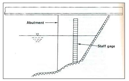
Fig. 21.1a. Staff Gauges.(Source: Singh, 1994)

Sometimes, a single gage is not adequate for all stages; a sectional staff gauge as shown in Figure 21.2, is used. Sectional gages are installed to provide overlap between various gages with their readings corresponding to the same datum.

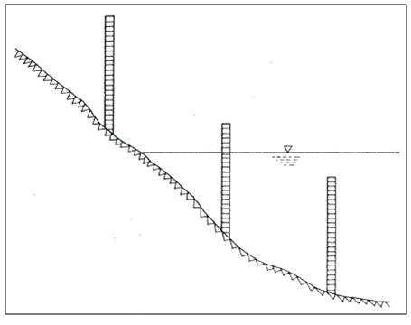
Fig. 21.1b.Sectional gauge.(Source: Singh, 1994)

A wire gauge measures the water-surface elevation from above such as from a bridge or other overhead structure. A weight is lowered from the structure until it reaches the water surface. The gauge has a drum with a circumference equal to 1 ft or 1 m of wire. The number of revolutions of the drum is measured by a mechanical counter, which, in turn, measures the length of the wire transmitted to reach the water surface. The operating range of a wire-weight gage is about 25 m.

 

21.1.2 Crest-stage Gauges

A special application of a staff-gage installation is the crest gauge. The crest gage is designed to obtain a measurement of the peak discharge in a channel reach during a flood event. A crest gauge consists of an ordinary staff gauge of sufficient width hand selected length to fit into a 2-inch galvanized pipe, as shown in Fig. 21.3. This galvanized pipe is fitted with threaded pipe caps on either end in which are drilled several holes of approximately 0.25 inch in diameter. The pipe is mounted vertically in the stream channel with it s bottom at the stream datum. The staff gage is inserted at the top of the pipe along with about a capful of ground cork and the top ventilated pipe cap is replaced.

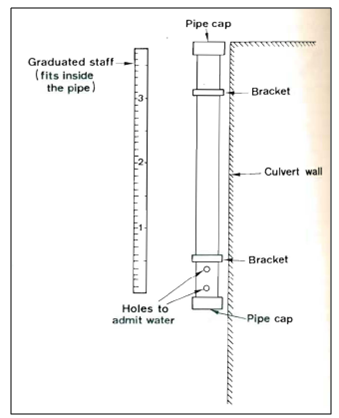
Fig. 21.3.Crest-staff gauge.(Source: Singh, 1994)

During a flood event, water enters the lower cap perforations and rises in the pipe, carrying the ground cork with it. At the highest stage, the cork adheres to the wetter staff, and as the water recedes, a visual record of the highest stage is indicated by the cork adhering to the staff. The operator only needs to remove the stall read the high stage and wipe the staff clean for additional use. Additional ground cork may be added, as necessary to replace that which is lost.

 

21.1.3 Recording Stream Gauges

Recording stream gages are instruments that continuously record the water stage at a given location along the stream. Two types are in general use: (i) the float type and (ii) the bubble gauge or manometer-servo water-level sensor.

 

a)  Float type gauge

The float-type recorder is shown in Fig. 21.4.

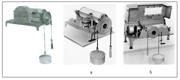
Fig. 21.4.Float-type gauge recorder: (Stevens’s type) (a) pen and chart type (b) digital.(Source: http://www.usbr.gov/pmts/hydraulics_lab/pubs/wmm/chap06_05.html)

The recorder is located in a stilling well that consists of a vertically mounted culvert or other similar structure that may be from 1 to 3 feet in diameter, as shown in Fig. 21.5. The culvert is installed on the .bank of the channel to a depth at least equal to the lowest level of the channel bottom. A 2-inch open-ended galvanized pipe is run horizontally from the bottom or near the bottom of the deepest part of the channel and fastened to the culvert. The top of this pipe is usually used as the stream-gage datum because it marks the lowest stage of streamflow or nearly so.

 

The recorder is mounted in a weatherproof housing at the top of the culvert and stilling well. Water rises in the stilling well through the 2-inch galvanized pipe to a level equal to the water elevation in the channel. The purpose of the stilling well is to dampen the water-surface fluctuations so that the float records changes in water elevation, but does not reflect wave action or other interference. Water-level changes are recorded on punched tape at selected time intervals, often every 15 minutes. This instrument can be adapted to remote monitoring by telephone or radio.

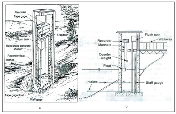
Fig. 21.5.Stilling well for float-type recorder (a) field installation (b) schematic.(Source: Singh, 1994)

Older recorders, from which many records exist, used a pen that marked stage elevations on a chart mounted on a clock-driven drum. These instruments required the chart to be changed periodically.

a)  Bubble gauge

The bubble gage, or manometer-servo water-level sensor, is shown in Fig. 21.6. This instrument eliminates the need for a stilling well, but requires battery power and a 116-ft³ dry nitrogen cylinder for operating up to 6 months.Pressure corresponding to the water head in the channel is imparted to the recorder through a tube in the bottom of the channel. This tube is supplied with nitrogen gas pressure equal to the water head by a servo motor that automatically adjusts for changes in water head. This instrument is attached to a digital recorder, similar to the float-type recorder, and can be remotely monitored by telephone or radio.

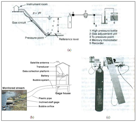
Fig. 21.6.  Bubble gauge recorder: (a) Schematic of bubble gauge installation (b) Field installation of bubble gauge (c) Bubble gauge: Stevens’s manometer servo.

(Source: http://nh.water.usgs.gov/gauge_station/3_howusgs.htm)(Singh, 1994)

The bubble gage may be preferable to the float-type recording gage for the following reasons:

1. The stilling well, which is expensive, is not needed.

2. Large changes (up to 30 m) in water-surface elevation can be measured.

3. The inlet is less likely to be blocked because of the gas pressure.

4. The recorder assembly can be located far away from the sensing point.

 

21.1.4 River-stage Data

The stage data are presented chronologically in time as a time series. Their plot, as shown in Fig. 21.7, is called a stage hydrograph. The primary use of this data is the determination of discharge. Other uses of this data are in flood-insurance studies, design of flood-protection works, flood warning and evacuation, urban development, flood-damage assessment, water diversion, navigation, etc. Long-term stage data are needed to estimate peak river stages for application in the design of hydraulic structures such as bridges, culverts, weirs, etc.

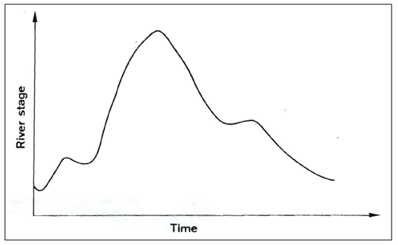
Fig. 21.7.Stage hydrograph.(Source: Singh, 1994)

 

21.2 Measurement of Velocity(Singh, 1994)

21.2.1 Velocity Distribution

Velocity distribution in a channel is not uniform over the width and depth of the channel. Velocity is greatest in the deepest part of the channel and is zero along the boundary of flow as shown in Fig. 21.8.

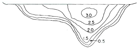
Fig. 21.8.Velocity distribution in a non-uniform channel.

(Source: Singh, 1994)

The greatest velocity occurs just under the water surface in the deepest part of the channel of a straight reach.

For computing the average vertical velocity of streamflow, following criterion is considered:

1.The average velocity in shallow streams with depths of flow not exceeding 3 m is taken as the velocity measured at 0.6 times the depth of flow, ,below the water surface,

(21.1)

This procedure needs a single-point measurement.

2.The average velocity in moderately deep streams is computed as

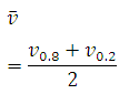 (21.2)

Where v_0.2 is the velocity measured at 0.2 times the depth of flow below the water surface andis the velocity measured at 0.8 times the depth of flow below the water surface.

 3. The average velocity in rivers having flood flows is obtained from a single measurement as

(21.3)

Where v_0.5 is the surface velocity measured within a depth of 0.5 m below the water surface; and c is a reduction factor, which is usually between 0.85 and 0.95, and is obtained from measurements taken at lower stages.

 

21.2.2 Estimating the Mean Channel Velocity of Floats

It is possible to estimate the mean velocity of flow in a channel, when necessary, by timing the movement of a float along a measured channel reach.

(21.4)

WhereL is the distance traveled in meters, and T is the time of travel in seconds.

 

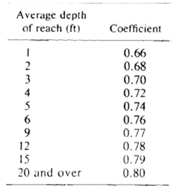
This method must be used in a straight reach of channel on a windless day so that the float can be maintained in the center of the channel. Because velocity varies across the width and depth of flow in the stream, coefficients must be applied to convert surface-float (Fig. 21.9) velocity to mean channel velocity. These coefficients, shown in Table 21.1., have been developed from empirical relations.

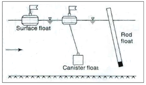
Fig. 21.9.Floats.(Source: Singh, 1994)

 

Table 21.1a. Coefficients for surface-float velocity measurements

(Source: Singh, 1994)

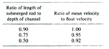
Somewhat better results are obtained when using a rod float(Fig. 21.9) 1 to 2 inches in diameter. The rod must be weighted on one end such that it floats vertically in the water and should be of such a length that the immersed length is 0.9 times the depth of water. Under these conditions, the rod tends to integrate the variations in vertical velocity distribution and tends to move at approximately the mean velocity. Table 21.2 gives coefficients for conversion of rod-float velocity to mean channel velocity.

 

Table 21.1b. Coefficients for rod-float velocity measurements

(Source: Singh, 1994)

 

21.2.3 Current Meters

The current meter is the most commonly used instrument to measure velocity of flow in streams.

 

It consists essentially of a rotating element which rotates due to the reaction of the stream current with an angular velocity proportional to the stream velocity.

There are two main types of current meters: (i) Vertical-axis meters, and (ii) Horizontal-axis meters.

 

1)  Vertical-Axis Meters

These instruments consist of a series of conical cups mounted around a vertical axis (Fig. 21.10. and 21.11.).

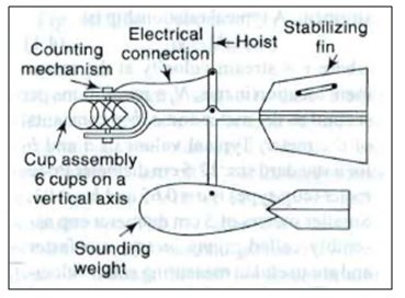
Fig. 21.10.Vertical-axis current meter. (Source: Subramanya, 2008)

 

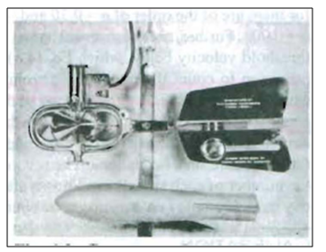
Fig. 21.11.Cup type current meter with sounding weight.

(Source: Subramanya, 2008)

The cups rotate in a horizontal plane and a cam attached to the vertical axial spindle records generated signals proportional to the revolutions of the cup assembly. The Price current meter and Gurley current meter are typical instruments under this category. The normal range of velocities is from 0.15 to 4.0 m/s.

 

The accuracy of these instruments is about 1.50% at the threshold value and improves to about 0.30% at speeds in excess of 1.0 m/s. Vertical-axis instruments have the disadvantage that they cannot be used in situations where there are appreciable vertical components of velocities.

 

(2) Horizontal-axis Meters

These meters consist of a propeller mounted at the end of horizontal shaft as shown in Fig. 21.12.  These come in a wide variety of size with propeller diameters in the range 6 to 12 cm, and can register velocities in the range of 0.15 to 4.0m/s. Ott, Neyrtec and Watt type meters are typical instruments under this kind. These meters are fairly rugged and are not affected by oblique flows of as much as 15°. The accuracy of tile instruments is about 1% at the threshold value and about 0.25% at a velocity of 0.3 m/sand above.

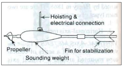
Fig. 21.12a.Horizontal-axis current meter. (Source: Subramanya, 2008)

A current meter is so designed that its rotation speed varies linearly with the stream velocity v at the location of the instrument. A typical relationship is

 (21.5)

Wherev is the stream velocity at the instrument location in m/s; N_s. = revolutions per second of the meter and a, b =constants of the meter.Typical values of a andb for a standard size 12.5 cm diameter Price meter (cup-type) (Fig. 21.13) is a = 0.65 and b=0.03. Smaller meters of 5 cm diameter cup assembly called pigmy meters run faster are useful in measuring small velocities. The value of the meter constants for them are of the order of a = 0.30 and b= 0.003.

 

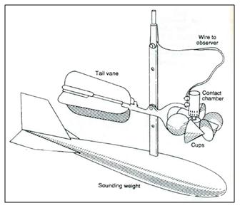
Fig. 21.12b.Price current meter.(Source: Singh, 1994)

 

21.3 Measurement of Discharge

21.3.1 Velocity-area Station Method

Velocity-area stations have stream gauges that measure velocities and cross-sectional areas of flow to obtain discharges. The basic equation used to obtain the discharge from velocity-area stations is

 (21.6)

WhereQ is the discharge in cubic meters per second (m³/s), V is the mean velocity of flow through the cross-sectional area of the channel in meters per second (m/s), and A is the cross-sectional area of flow in square meters (m²). Equation 21.6 can be used as a continuity equation because the mass flow into a point must equal the mass flow out from that point. To determine the discharge both the mean velocity and cross-sectional area of flow must be measured.

In order to conduct stream-discharge measurements, the stream channel must be subdivided into several smaller widths. The vertical dashed lines in Fig. 21.13 represent subdivisions of the stream width.

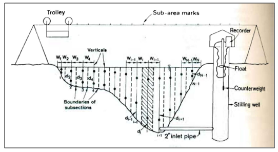
Fig. 21.13.Schematic sketch of a velocity-area station.(Source: Singh, 1994)

The average velocity in each of the sub-width divisions is measured. The mean depth of flow of this subdivision is measured using sounding rods, sounding weights or an echo-depth recorder (an electroacoustic instrument). A current meter is used to measure velocity for this subdivision. Velocity is measured from observations at points 0.2 and 0.8 of the total depth. These two velocity measurements are averaged to obtain the mean velocity in that subwidth. The discharge for the subdivision is computed by taking the product of the mean depth, subarea width and mean velocity. Equation 21.6 is applied to the subdivision. Total discharge for the stream is determined by summing the discharges for all subwidths. The mean stream velocity can be computed by dividing the total discharge by the total cross-sections area. The velocity-area method when using the current-meter method is also referred to as the standard current-meter method.

 

Calculation of Discharge

Fig. 21.13 shows the cross section of a river in which N -1 verticals are drawn. The velocity averaged over the vertical at each section is known. Considering the total area to be divided into N -1 segments, the total discharge is calculated by the method of mid-sections as follows.

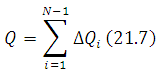
Where ΔQ in the i th segment

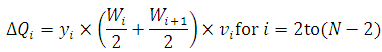 (21.8)

 

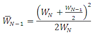
For the first and last sections, the segments are taken to have triangular areas and area calculated as

Where

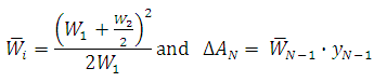(21.10)

(21.11)

 (21.12)

 

 

21.3.2 Moving Boat Method

Discharge measurement of large alluvial rivers, such as the Ganga, by the standard current meter is very time consuming even when the flow is low or moderate. When the river is in spate, it is almost impossible to use the standard current meter technique due to the difficulty of keeping the boat stationary on the fast-moving surface of the stream for observation purposes. It is in such circumstance that the moving boat techniques prove very helpful.

 

In this method a special propeller-type current meter which is free to move about a vertical axis is towed in a boat at a velocity v_bat right angles to the stream flow. If the flow velocity is v_fthe meter will align itself in the direction f resultant velocity v_Rmaking an angle θwith the direction the boat (Fig. 21.14).

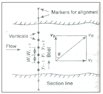
Fig. 21.14.Moving-boat method. (Source: Subramanya, 2008)

Further, the meter will register the velocity v_R. If v_b is normal to v_f,

 

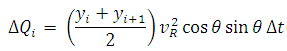
If the time of transit between two verticals is Δt, then the width between the two verticals (Fig. 21.14) is

 

The flow in the sub-area between two verticals i and i + 1 where the depths are y_i and y_i+1respectively, by assuming the current meter to measure the average velocity in the vertical, is

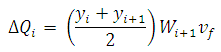
i.e.

 (21.13)

 

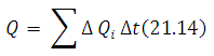
Thus by measuring the depths y_i, velocity v_Rand θ in a reach and the time taken to cross the reach Δt, the discharge in the sub-area can be determined. The summation of the partial discharges ΔQ_i, over the whole width of the stream gives the stream discharges

 

21.3.3 Chemical Gauging

Chemical gauging is also referred to as the dilution method and is especially useful in very small streams mountain streams strewn with boulders, etc. This method employes the conservation of mass of the tracer to be used. Common salt, fluorescent dyes and radioactive materials are the main tracers used. A tracer should be able to mix freely with flow; should not react with sediment, channel boundaries, or vegetation: and should not evaporate. The tracer of specified concentration C₁,is injected into the stream at a constant rate Q_tat a defined location. Samples are taken at a downstream point where the concentration gradually rises to a constant value C₂ as shown in Fig. 21.15.

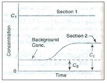
Fig. 21.15.Constant rate injection method. (Source: Subramanya, 2008)

Let C₀be the initial concentration of tracer in the stream. At steady state, the mass conservation for the tracer between the two locations can be expressed as

i.e.

(21.15)

This technique in which Q is estimated by knowing C₁C₂, C₀ and Q_t, is known as constant rate injection method or plateau gauging.

 

 

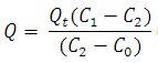
21.3.4 Ultrasonic Method

In this method (Fig. 21.16), ultrasonic signals are used to measure flow velocity. Two transducers are installed at the same elevation from the bed on both sides of the stream. The path connecting the transducers makes an .angle with the direction of flow. The transducers receive as well as transmit ultrasonic signals. The time taken by a signal from one transducer to the other is recorded. The average velocity of flow along the path is then obtained by knowing the path length and its angle with the flow direction. This method of gauging is suitable for automatic recording of data. It is accurate, efficient, and can accommodate rapid changes in the magnitude and direction of flow. However, unstable cross-sections, large loads of sediment in suspension, steep temperature changes, changing weed growth, air entrapment, changes in salinity, etc., can reduce accuracy of this method.

Fig. 21.16.Ultrasonic method. (Source: Subramanya, 2008)

 

21.3.5 Electromagnetic Method

The electromagnetic method is based on the Faraday's principle that an emf is induced in the conductor (water in the present case) when it cuts a normal magnetic field. Large coils buried at the bottom of the channel carry a current 1 to produce a controlled vertical magnetic field (Fig. 21.17)

 

Electrodes provided at the sides of the channel section measure tbe small voltage produced due to flow of water in the channd.1t has been found that the signal output E will be of the order of millivolts and is related to the discharge Q as

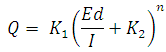 (21.16)

Whered is depth of flow, Iis current in the soil, and n, K₁and K₂ are system constants.

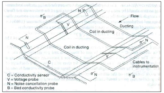
Fig. 21.17.Electromagnetic method. (Source: Subramanya, 2008)

Present day commercially available electromagnetic flowmeters can measure the discharge to an accuracy of ±3%, the maximum channel width that can be accommodated being 100 m. The minimum detectable velocity is 0.005 m/s.

 

21.3.6 Indirect Method

These methods measure flow depths at specified locations, and translate these depths into discharges using depth-discharge relations applicable to those locations. Flow-measuring structures and slope-area methods exemplify indirect methods.

 

Flow Measuring Structures

Different types of flow-measuring structures are in use. Broad-crested weirs, flumes made of concrete, masonry or metal sheets, and V-notches are common examples of such structures. When a flow-measuring structure is installed in a stream, it produces a unique control section in the flow. The discharge Q through the structure is related to the water-surface elevation H adjacent to or within the structure as

Q = f (H)  (21.17)

Where f is some function

For example, for a weir

in which B is the width of the weir crest, C is the discharge coefficient, and x is an exponent. Both C and x are specific for a weir, and are obtained by calibration.

 

The value of C takes into account the channel geometry, the friction loss due to the weir, horizontal and vertical contractions of flow, the form of the weir, etc.

 

Slope-area Method    

This method is based on the principle of energy conservation. A stream reach is selected, as shown in Fig. 21.18. From Bernoulli’s equation applied to the ends of the reach (sections t and 2),

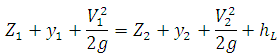 (21.19)

Where is head loss in the river reach.The head loss h_Lcan be considered to be made up of two parts (i) frictional loss h_fand (ii) eddy loss h_e.Denoting Z + Y = h = water surface elevation above the datum,

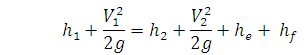
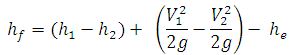 (21.20)

 

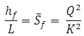
If L is length of the reach, by Manning's formula for uniform flow,

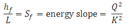
In non-uniform flow an average conveyance is used to estimate the energy slope and

where K = conveyance  of channel = 

n = Manning’s coefficient

The eddy loss h_eis estimated as

 (21.21)

Where

n= Manning’s coefficient

The eddy loss h_eis estimated as

 

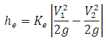
where    K_e= eddy-loss coefficient having values as below.

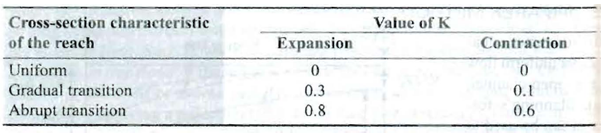
Equation (21.20), (21.21) and (21.22) together with the continuity equation Q = A_lV₁ = A₂V₂ enable the discharge Q to be estimated for known values of h,channel cross-sectional properties and n.

 

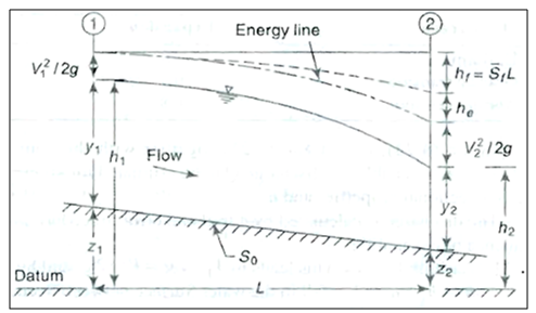
Fig. 21.18.Slope-area method. (Source: Subramanya, 2008)

 

21.4 Rating Curve

A stage-discharge relation for a velocity-area station or gauging section is obtained by plotting measured stage on the ordinate and the measured discharge on the abscissa as shown in

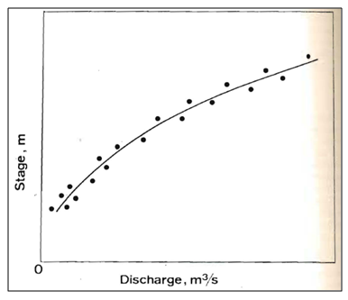
Fig. 21.19. This relation is also called the rating curve.

Fig. 21.19.Stage-discharge relationship.(Source: Singh, 1994)

It represents the integrated effect of a wide range of channel and flow parameters. The combined effect of these parameters is designated as control. If the rating curve for a gauging station does not change with time the control is called permanent; otherwise, 'it is called shifting control. The stage-discharge relation is of fundamental importance in the acquisition of discharge measurements. All direct discharge-measuring methods require construction of this relationship before measured stages can he translated into' discharges.

 

21.4.1 Simple Rating Curve

A majority of streams and rivers, especially non-alluvial rivers exhibit permanent control. For such a case, the relationship between the stage and the discharge is a single valued relation which is expressed as

  (21.23)

 

WhereQ is stream discharge, G is gauge height (stage), ais a constant representing the gage reading for zero discharge, and and  are rating curve constants.

 

Equation 21.20 is called the rating equation of stream and can be used for estimating the discharge Q of the stream for a given gauge reading G within range of data used in its derivation.

 

When the data are plotted on logarithmic paper the plot is a straight line, as shown in Fig. 21.20.Equation 21.23becomes

  (21.24)

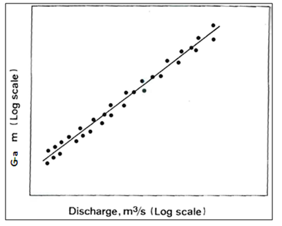
Fig. 21.20.Stage-discharge relationship on logarithmic paper.

(Source: Singh, 1994)

The best values of constants and can be obtained using the least square, method.

1. Constant a must be found beforehand, and this can be estimated using following methods.

2. Trial and error method.

3. To extrapolate the rating curve corresponding to Q = 0 and then plot log Q versus log (G-a).

4. Analytical method.

The simple rating curve is generally satisfactory for a majority of streams where rapid fluctuations of stage are not experienced at the gauging section. The adequacy of the curve is measured by the scatter of data around the fitted curve. When there is a permanent control, the rating curve is essentially permanent. If the rating curve is made using a range of stages from low to high, it can be used to interpolate the discharge for any stage of flow between the measured stages without measuring that flow. It is important to check the stability of the curve by periodic discharge measurements, and to extend it with each new observed high stage. Changes in channel shape, due to scouring or sedimentation, can change the effect of control and thereby change the rating curve.

 

21.4.2 Shifting Control

When the control of a gauging station changes, its rating curve changes. The change may result from (1) scour or deposition, (2) varying back water, (3) rapidly changing flow, and (4) changes in flow caused by dredging, channel encroachment and weed growth, etc. For the shifting control due to cases (1) and (4), frequent current meter gauging is needed. The discharge is then estimated by noting the difference between the stage at the time of a discharge measurement and the stage obtained from the rating curve corresponding to the same discharge. This difference serves as a correction and is applied to all stages before reading the rating curve. If this correction varies from one measurement to another, it can be assumed to vary linearly in time. The effect of backwater and unsteady flow is amenable to analytical treatment.

 

21.4.3 Constant-fall Rating Curve

The backwater may develop as a result of an obstruction downstream or high stages in an intersection stream, and may be variable in time. Under the condition of shifting control due to backwater effects, a given stage will indicate different discharge values. This results from differences in water-surface slope at the control. The discharge is estimated by establishing another gage some distance downstream of the main gauging station. This other gage is called the secondary, or auxiliary, gage. Measurements are made at both gages.

 

The difference between stages of these gages indicates the fall (F) or slope (S = F/L) of the water surface in the reach.

The discharge then is a function of stage G (at the main gage) and fall F, and is expressed as

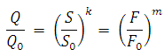 (21.25)

 

Whereis the normalized discharge at the stage when  = or , and k and m are exponents.

 

This method is called the slope-stage-discharge rating-curve method.

 

All observed values of stage and discharge for values of F = F₀ are plotted as a simple rating curve, as shown in Fig. 21.21. This is the Q₀ versus G curve and is called the constant-fall curve.

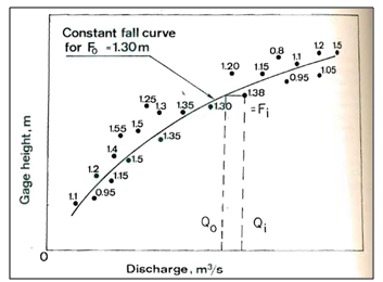
Fig. 21.21.Constant-fall rating curve.(Source: Singh, 1994)

For each measurement with F ≠F₀, values of Q/Q₀and F/F₀are calculated and plotted as shown in Fig. 21.22. The plot of Q/Q₀versus F/F₀is called the auxiliary curve or adjustment curve.

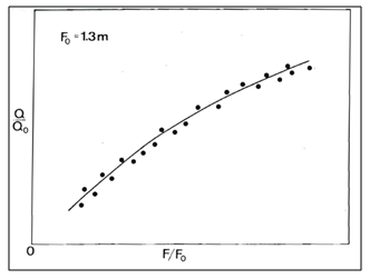
Fig. 21.22.Adjustment curve for constant-fall rating curve.

(Source: Singh, 1994)

 

21.4.4 Normal-fall Rating Curve

Under some conditions, Fvaries widely and its variation is related to stage. Then a normal fall, F_n, is defined as a function of stage, which replaces F₀in Eq. (21.25), as shown in Fig. 21.23. This is a second auxiliary curve. Correspondingly, normal Row Q_nreplaces Q₀.

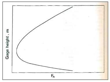
Fig. 21.23.Normal-fall rating curve.(Source: Singh, 1994)

Correspondingly, normal flowQ_nreplacesQ₀. Analogous to a constant-fall rating, a normal fall rating is employed, as shown in Fig. 21.24.

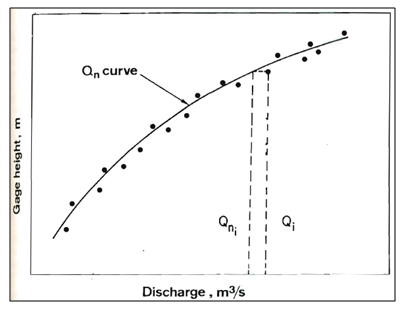
Fig. 21.24.Q_n for normal-fall rating curve.(Source: Singh, 1994)

In the same vein, the auxiliary curve is obtained by plotting Q/Q_nversus F/F_nas shown in Fig. 21.25.

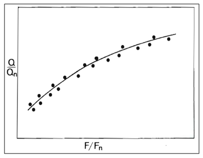
Fig. 21.25.Auxiliary curve for normal-fall rating curve.(Source: Singh, 1994)

For a given stage, the value of actual fall F is computed first. Then a value of F_nis obtained from the second auxiliary curve, and the ratio F/F_nis computed. Against this value of F/F_n, the value of Q/Q_nis obtained from the first auxiliary curve. The value of Q_nis read from the raring curve, which then is multiplied by Q/Q_nto yield the actual value of discharge, that is, Q = (Q/Q_n)x Q_n.

 

21.4.5 Loop Rating Curve

During the passage of a flood past a gauging section, the stage-discharge relation for the rising limb of the hydrograph is different from the one for the falling limb. During the rise of flood, the velocity and discharge are greater for a given stage than they are for the same stage when the flow is steady and uniform. During the falling stage, the reverse is true. Thus, the stage-discharge relation for unsteady flows is a loop, as shown in Fig. 21.26.

Fig. 21.26.Stage-discharge relationship for unsteady flow.(Source: Singh, 1994)

It may be seen that for the same stage, there is greater discharge through the stream reach during the rising stage than it is during the falling stage. This loop may be plotted from stage and discharge measurements of a flood. This curve can be used as an approximation for other floods of about the same magnitude and duration.

 

For floods with multiple peaks, the loop may be complicated. Thus, a better procedure is to relate for the same stage the normal discharge, Q_Nunder steady uniform flow to the measured unsteady-flow discharge Q_M (Chow. 1959) as

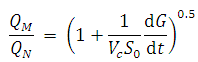 (21.26)

Whereis the velocity of the flood wave or wave celerity;  is the channel slope, the slope of the water surface for uniform flow, and dG/dtis the rate of change of the stage.

  

References

Singh, V. P.(1994). Elementary Hydrology. Prentice Hall of India Private Limited, 377-427.

Subramanya, K. (1994). Engineering Hydrology.Third edition, Tata McGraw Hill, 101-131.

 

Suggested Reading

Murty, V.V.N. and Jha, M.K. (2009).Land and Water Management Engineering.Fifth edition, Kalyani Publishers, Ludhiana.