Farm Machinery and Equipment-II 3(2+1)

LESSON 32. MANAGEMENT OF FARM MACHINERY; REPLACEMENT, BREAK-EVEN POINT ETC

SELECTION OF TRACTOR

A successful farm machinery system is one that must perform in such a manner that profit to the farm is maximized. Maximization is not always accomplished by minimizing costs, and such is true with the selection of a farm machinery system. Considerations have to be given to the economic value of operating machinery at that correct moment in time when the soil, the crop, the weeds, and the insects are most affected. The need for timely operations is a rather unique economic constraint on the farm machinery system. Agronomic practices, enterprise and topographic variability require that machinery selection must be made on an individual farm basis. This requirement implies that such a programme must be adaptable to a large number of input data and should accommodate many special circumstances. Machine capacity can be described as:

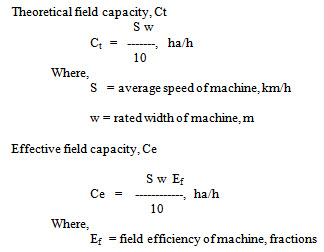
Selection of an appropriate machinery system may be stated simply as the process of determining those individual machine capacities, which will optimize the economic performance of the whole system. Consideration must be given to machine costs, power costs, operational costs etc.  An appropriate cost of operation model is essential to the validity of the selection problem analysis. This analysis uses fixed and variable costs.  Variable costs increase proportionally with the operational use of the machine, while fixed costs are independent of use.  Considering the fixed and variable cost, the total cost of operation of tractor is given by

            Ac       =          Fc Pt  +  At ( RM + L + O + F + Tc )      ------------  (1)

Where,

            Ac       =          Annual costs of operating the tractor, Rs/Yr.

            Fc        =          Annual fixed costs, fraction of purchase price

            Pt         =          Purchase price of tractor, Rs

            At        =          Annual use of tractor, h/Yr.

            RM      =          Repair and maintenance costs of tractor, Rs/h

            L          =          Labour costs, Rs/h

            O         =          Oil costs, Rs/h

            F          =          Fuel costs, Rs/h

            Tc        =          Timeliness costs, Rs/h

            Yr        =          Year

Since RM, O, F = f (A) where A is cropped area, therefore, RM, O, F = f (E) where E is energy spent to cover the area. As energy requirement is expected to be a constant for a specific farm operation, therefore, RM, O and F costs will have no influence on the optimum size of the tractor. Thus, only important variables are labour costs (L) and timeliness costs (Tc) . More specifically, the annual costs of tractor is expressed as the sum of the fixed costs and the total labour and timeliness costs for each of two types farm jobs viz. field operations and transport operations.

    Ac  = Fc Pt  +  (Field hours) (L+ timeliness cost) + (transport hours) (Lt) ------- (2)

Where,

            L          =          Tractor operator’s wages for field work, Rs/h

            Lt        =          Labour cost for transport work, Rs/h

Probably, there should be a timeliness charge for transport work but for simplicity it may be assumed that this does not limit field operation.

The optimum size of tractor is considered to be one, which will perform all the desired operations at minimum costs.  The annual hours of work required for each class of tractor operation are given by:

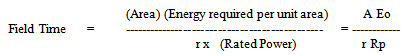
Where,

                        A         =          Area

                        r           =          Ratio of drawbar power to rated engine power for drawbar loads and ratio of PTO power to rated engine power for PTO  loads.

                        Eo        =          Energy required per unit area

                        Rp       =          Rated power

Thus field time is proportional to energy required per unit area per rated power i.e.

Field Time = C₁ Eo / Rp

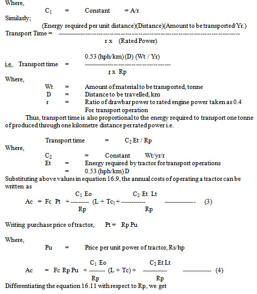
(RP)_opt    =       [{1/ (Fc Pu)} {C₁ Eo (L +Tc) + C₂ Et Lt}]^1/2        ------------  (5)

Differentiating equation 5 once again w.r.t. Rp, we get 

 

d (Ac)                          2 C₁ Eo (L + Tc)                 2 C₂  Et  Lt

--------              =          ---------------------      +     --------------------

d (Rp)²                                    (Rp)³                                (Rp)³

 Which is a positive quantity, indicating that the calculated (RP)opt  would have a minimum cost of operation.

Timeliness of a field operation must be considered in selection of optimum power required of a tractor.  Total timeliness cost for an operation depends upon the scheduling of operations (delayed, premature and balance).  So, the total timeliness cost (Tc) can be estimated as:

                                                    K Y V A²

                                    Tc   =   ---------------             --------------- (6) 

                                                     X U Z

Where,

            Tc        =           Timeliness costs,  Rs./h

            K         =           Timeliness loss factor

            Y         =           Crop yield, t/ha

            V         =           Value of crop, Rs./t

            A         =           Total area under crop, ha

            U         =           Ratio of total working days to total days, fraction

            Z          =           Effective machine capacity, ha/day

            X         =           2 for premature or delayed scheduling

                        =           4 for balanced scheduling

 Total timeliness costs for an operation depend on the scheduling of operations with respect to time and duration of operation.  There are basically three types of scheduling of operations viz. Delayed, premature and balanced.  In delayed scheduling, operation starts at optimum time whereas operation is planned to be completed by the optimum time in premature scheduling.  In the balanced scheduling, operation is planned in such a way that it spreads over equally on both sides of the optimum time.  Therefore, time devoted in case of delayed and premature scheduling is half of that of balanced scheduling.  Thus, X is taken as 2 for premature or delayed and 4 for balanced scheduling.

The cost of untimely operations can be included in the basic cost model as a cost for each hour the machine is used.  The absolute costs depend on the value of the crop. Therefore, a relative timeliness factor called K has been developed to give some generality to the analysis (Table 1). K is defined as the decimal reduction of the quantity and quality of the potential crop per hour of machine operation.

 Table 1: Timeliness loss factor for different operations and crops under Indian conditions

Crop	Operation	K value
Wheat	Tillage & sowing	0.00456
	Harvesting & threshing	0.00650
Barley	Tillage & sowing	0.0067
	Harvesting & threshing	0.00437
Paddy	Tillage & sowing	0.00625
	Harvesting & threshing	0.0066
Maize	Tillage & sowing	0.0047
Soybean	Tillage & sowing	0.0179
	Harvesting & threshing	0.0189
Moong	Tillage & sowing	0.0052
	Harvesting & threshing	0.066
Oil seeds	Tillage & sowing	0.0138
	Harvesting & threshing	0.0351

 

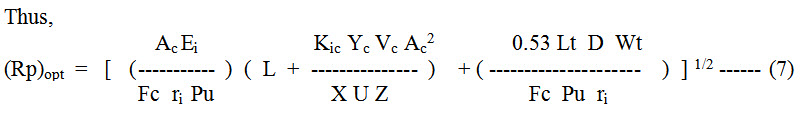
 Where,

Fc        =          Fixed cost percentage of a tractor

Pu       =          Price per unit power of tractor, Rs/hp

A_c        =          Area under crop, ha.

E_i         =          Energy required for operating an implement for a particular crop

K_ic       =          Timeliness loss factor of an implement for a particular crop

Yc       =          Yield of crop, q/ha

V_c        =          Value of crop, Rs./q

X         =          Constant equal to 2 for premature or delayed schedule and 4 for Balanced schedules

U         =          Fractional utilization of time

Lt        =          Labour rate for transportation, Rs./h

D         =          Distance to be traveled, km.

Wt       =          Weight to be transported, t

r_i          =          Ratio of drawbar power to rated engine power for drawbar load and ratio of PTO power to rated engine power for PTO loads for a particular crop

Note that repairs, fuel and oil costs have been dropped from considerations. Only labour and tractor fixed costs remain in the equation 16.14.  Equation 16.14 may be used without reservation for self-propelled implements and for selection of implements to fit into an existing machinery system where the tractor fixed costs are known and are constant. In fact, the optimum implement width may be more dependent upon the size of tractor than upon any of the other factors in equation 16.14.  Selection of an economic system of machines is highly dependent upon the horsepower level of the tractor or tractors.

REPLACEMENT OF FARM MACHINERY

Good guidelines are available for making management decisions on when to replace the farm equipment. Important reasons for replacing a machine are:

i) Accidents have damaged the implement beyond repair

ii) Field capacity of the machine is inadequate

iii) A new machine or farm practice has made the old machine obsolete

iv) Performance of a new machine is significantly superior

v) Anticipated costs for operating the old machine exceed those for a replacement machine, and

vi) The machine is worn out.

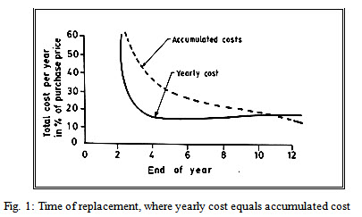
The time of replacement decisions depends on the accumulated costs over a period of years. The annual cost curve as well as the accumulated average cost curve for a machine is shown in Fig. 1. Both the curves intersect at a point. Theoretically, the time to replace a machine is when the annual cost starts to exceed the average accumulated cost. However, machine repair rate really determines the time of replacement. One method of establishing the time of replacement is to determine that the cost per unit of use has reached its lowest value.

Case I: Repair is proportional to use

Total cost,       C         = FC + RC X

Where,

C         = Total repair cost

FC       = Fixed cost

RC       = Repair cost

X         = Number of ha of machine used

 

In this case, the lowest cost/ha can only be attained with indefinite use of machine as shown in Fig. 2.

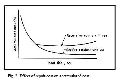
Case II: Repair cost increases with use

C = FC + R₁ C X + R₂ C X²

Where,

C         = Total repair cost

FC       = Fixed cost

R₁C     = Repair cost rate proportional to use

R₂C     = Repair cost rate that increases with use

X         = Number of hectare of machine use

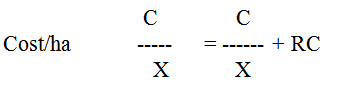
Repair cost per hectare is given by

 C             FC

----       = ------- + R₁C + R₂C X 

 X              X

The time of replacement is defined by the minimum cost point. If replacement is delayed beyond this point, costs are expected to rise due to the increasing repair cost.

For minimum cost

  Or,     X         = [ FC/R₂C ]^1/2

The accumulated repair cost will depend upon the type of repair rate. For constant repair rates, the effect of repair on replacement is ignored. For implements, which have an increasing repair rate, the repair cost is given by

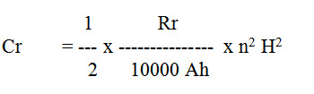
Where,

Cr        = Accumulated repair cost up to Year n, Rs

Rr        = Value of repair rate at a given accumulated hours of use, expressed 

                in %P/100 hours

P          = Purchase price, Rs

Ah       = Accumulated hours

H         = Average hourly use per year

Obsolescence should be considered in determining the proper time of replacement. Accumulated cost of obsolescence can be expressed as

Co = 1/2 (Fo n²)

Where,

Co       = Accumulated cost of obsolescence, Rs

Fo        = Obsolescence factor, Rs/year

N         = Number of years

In this case, the depreciation can be expressed in terms of percentage of purchase price at the beginning of year n as

Vn       = 68 - 4.2 n                  for tractors

Vn       = 60 - 4.6 n                  for other implements

Where,

Vn       = Remaining value at any time, Rs

n          = Number representing age of machine in years at the

               beginning of year in question

The accumulated depreciation cost can be calculated as

Cd       = (100 -Vn) %P

Where,

Cd       = Accumulated depreciation cost up to year n, Rs

P          = Purchase price, Rs

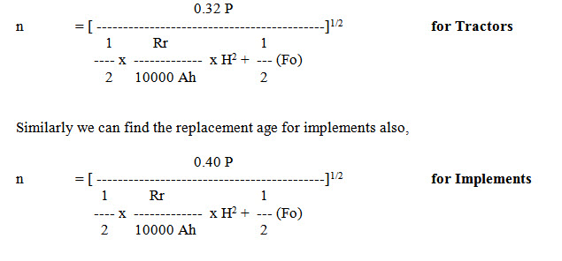
Optimum replacement time (n) would be in the year when the total accumulated cost of depreciation; repair and obsolescence per year would be the minimum and can be calculated by:

BREAK-EVEN USE

Hiring custom operators is one important alternative to owing machinery. In some cases, using custom operators provides faster completion of work provides the least-cost method and does not require the capital needed for owing a machine. But when considering hiring a custom operator, do not forget timeliness of operations. Waiting for a custom operator to arrive is expensive in terms of timeliness, if it means not getting crops planted or harvested at the optimum time. Always consider timeliness in making a decision to use either a custom operator or an alternative method.

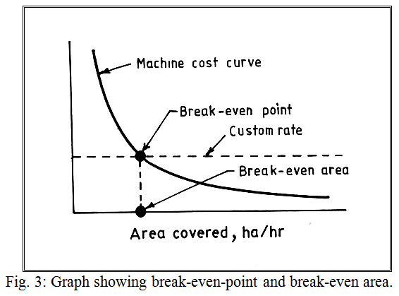
Determining when to use a custom operator is one of the most important decisions made in machinery management. To take a decision in this regard, the knowledge of break-even-use of a farm machine is a must. The break-even-use is the amount of use where the cost of using a machine owned would be the same as the cost of hiring a machine (Fig. 3). If a machine were used for less than the break-even-use, custom rate would be profitable. Otherwise owning a machine would be profitable.

Break-even-use can be determined by the following formula:

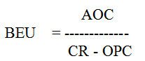
Where,

BEU    = Break-even-use, ha

AOC   = Annual ownership cost (fixed cost), Rs

CR       = Custom rate, Rs/ha

              OPC    = Operating costs, Rs/ha

UTILITIES AND RELIABILITY INDEX

Utility index: It is a direct indication of work machine contact hours. With an increase in the utility index the cost of operation and the non-operating hours decrease. This in turn, results into a net increase in the total power available for farm work. Utility index (K) can be calculated as

                      Number of actual working hours/year

K         = --------------------------------------------------------

                     Number of expected working hours/year

Reliability index: This index measures the percentage of assurance of proper working of tractors. It is determined as follows:

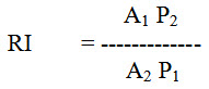
Where,

RI        = Reliability index

A₁        = Breakdown charges available = 0.04 nP

A₂        = Breakdown charges - actual incurred

P₁         = Penalty for breakdown = 0.25 x 10^-3 B P

P₂         = Money blocked in storing the requisite spare parts

P          = New cost of tractor

n          = Number of years of breakdown occurrence since purchase

B         = Number of breakdown hours

Thus,

                    0.04 n P              P₂                   160 n P₂

RI        = ---------------- x --------------- = -------------------

                 0.25x10^-3            B P A₂                  B A₂

The optimum reliability index is determined by assuming P₂/A₂ = 1. Although P₂/A₂ is not exactly equal to 1 and it keeps on fluctuating but in an Indian condition through previous experience it has been observed that on an average P₂ is more or less equal to A₂. Thus, above equation can be rewritten as

If we take reliability index 1, then B = 160 n

If n = 15 years for tractor

B = 160 x 15 = 2400 hours

This indicates that in order to maintain an optimum reliability index, the total number of breakdown hours in the life time of tractor must not exceed 2400 hours.