Mechanics of Tillage and Traction 3(2+1)

LESSON 31. GEOSTATISTICS / KRIGING

It is not uncommon to use probabilistic and statistical methods for describing partly known (or sampled) natural parameters.   Time series analysis is one of the earlier fields where variability has been considered and described with stochastic methods. These methods were extended and further developed to analyse spatial variability. These spatial methods form the discipline called geostatistics.

Geostatistics is a tool to help us characterize spatial variability and uncertainty resulting from imperfect characterization of that variability.  In its broadest sense, geostatistics can be defined as the branch of statistical sciences that studies spatial/temporal phenomena and capitalizes on spatial relationships to model possible values of variable(s) at unobserved, unsampled locations (Caers, 2005).

31.2 Objectives of geostatistics

• To find out the weighted average of any property which varies from point to point over a given area of land for result interpretation and for carrying out simulation experiments in the field.

• To work out interpolated values of a given property over time and space in unsampled or unvisited sites between sampled estimates for the purpose of depicting contour lines on the base maps.

31.3 Utilities of geostatistics

• Determination of the exact point at which maximum variability of a given property, under a given set of conditions, may be encountered.

• Mapping of a given area for a particular property can be accomplished in the most economical way, without actually surveying the entire area on a point basis.

• The results can most suitably be extended to development of stochastic models for any given property.

• The technique can help in conservation of resources by way of simply extrapolating the results on spatial analysis in a given sampling unit(s) to similar units established or reported elsewhere.

31.4 Basics of Geostatistics

Geostatistics involves the theory of regionalized variables, which dates back to the early fifties when in South-Africa D. Krige and his colleagues started to apply statistical techniques for ore reserve estimation. In the sixties, the French mathematician G. Matheron gave theoretical foundations to these methods. 

Application of Geostatistics in its nascent stages was oriented towards the mining industry, as high costs of drillings made the analysis of the data extremely important. Books and publications on geostatistics are mostly oriented to mining problems. The phenomenal growth of computer era has lead to affordable and cheaper computational methods and hence scope of geostatistics has drastically widened. Of late, applications of geostatistics can be found in very different disciplines ranging from the geology to soil science, hydrology, meteorology, environmental sciences, agriculture and even structural engineering.

Typical questions of interest to a geostatistician are (Hengl, 2009):

• How does a variable vary in space-time?

• What controls its variation in space-time?

• Where to locate samples to describe its spatial variability?

• How many samples are needed to represent its spatial variability?

• What is a value of a variable at some new location/time?

• What is the uncertainty of the estimated values?

Geostatistics are based on the concepts of regionalized variables, random functions, and stationarity. A brief theoretical discussion of these concepts is necessary to appreciate the practical application of geostatistics.

31.4.1 Regionalized variable and random function

A regionalized variable is the realization of a random function. This means that for each point u in the d dimensional space the value of the parameter we are interested in, z(u) is one realization of the random function Z(u). This interpretation of the natural parameters acknowledges the fact that it is not possible to describe them completely using deterministic methods only.  In most cases it is impossible to check the assumption that the parameter is the realization of a random function as we have to deal with a single realization.

31.4.2 Stationarity

A random function  Z(x) is said to be first-order stationary if its expected value is the same at all locations throughout the study region.

E (x) = m ... (1)

Where, m is the mean of classical statistics, and

      E Z (x) - Z ( x - h ) = m ...(2)                                         

Where, h is the vector of separation between sample locations.

Geostatistical methods are optimal when data are

• normally distributed and

• stationary (mean and variance do not vary significantly in space)

Significant deviations from normality and stationarity can cause problems, so it is always best to begin by looking at a histogram or similar plot to check for normality and a posting of the data values in space to check for significant trends.

There are three scientific objectives of geostatistics (Diggle and Jr, 2007):

1. Model estimation, i.e. inference about the model parameters;

2. Prediction, i.e. inference about the unobserved values of the target variable;

3. Hypothesis testing;

Model estimation is the basic analysis step, after which one can focus on prediction and/or hypothesis testing. In most cases all three objectives are interconnected and depend on each other. The difference between hypothesis testing and prediction is that, in the case of hypothesis testing, we typically look for the most reliable statistical technique that provides both a good estimate of the model, and a sound estimate of the associated uncertainty. It is often worth investing extra time to enhance the analysis and get a reliable estimate of probability associated with some important hypothesis, especially if the result affects long-term decision making. The end result of hypothesis testing is commonly a single number (probability) or a binary decision (Accept/Reject). Spatial prediction, on the other hand, is usually computationally intensive, so that sometimes, for pragmatic reasons, naïve approaches are more frequently used to generate outputs; uncertainty associated with spatial predictions is often ignored or overlooked. In other words, in the case of hypothesis testing we are often more interested in the uncertainty associated with some decision or claim; in the case of spatial prediction we are more interested in generating maps (within some feasible time-frame) i.e. exploring spatio-temporal patterns in data.

Spatial prediction or spatial interpolation aims at predicting values of the target variable over the whole area of interest, which typically results in images or maps. In geostatistics, interpolation corresponds to cases where the location being estimated is surrounded by the sampling locations and is within the spatial auto-correlation range. Prediction outside of the practical range (prediction error exceeds the global variance) is then referred to as extrapolation. In other words, extrapolation is prediction at locations where we do not have enough statistical evidence to make significant predictions.

An important distinction between geostatistical and conventional mapping of environmental variables is that geostatistical prediction is based on application of quantitative, statistical techniques. Until recently, maps of environmental variables have been primarily been generated by using mental models (expert systems). Unlike the traditional approaches to mapping, which rely on the use of empirical knowledge, in the case of geostatistical mapping we completely rely on the actual measurements and semi-automated algorithms.

In summary, geostatistical mapping can be defined as analytical production of maps by using field observations, explanatory information, and a computer program that calculates values at locations of interest (a study area). It typically comprises:

1. Design of sampling plans and computational workflow

2. Field data collection and laboratory analysis

3. Model estimation using the sampled point data (calibration)

4. Model implementation (prediction)

5. Model (cross-)evaluation using validation data

6. Final production and distribution of the output maps

31.4.3 Spatial Prediction Models

Spatial prediction models (algorithms) can be classified according to the amount of statistical analysis i.e. amount of expert knowledge included in the analysis:

31.4.3.1 Mechanical (Deterministic) Models

These are models where arbitrary or empirical model parameters are used. No estimate of the model error is available and usually no strict assumptions about the variability of a feature exist. The most common techniques that belong to this group are:

1. Thiessen polygons;

2. Inverse distance interpolation;

3. Regression on coordinates;

4. Natural neighbors;

5. Splines;

31.4.3.2 Linear Statistical (Probability) Models

In the case of statistical models, the model parameters are commonly estimated in an objective way, following probability theory. The predictions are accompanied with an estimate of the prediction error. A drawback is that the input data set usually needs to satisfy strict statistical assumptions. There are at least four groups of linear statistical models:

• kriging (plain geostatistics)

• environmental correlation (e.g. regression-based)

• Bayesian-based models (e.g. Bayesian Maximum Entropy)

• hybrid models (e.g. regression-kriging)

31.5 Kriging

Most geostatistical studies in natural resources management aim at estimating naturally occurring phenomena at unsampled places and mapping them.  Kriging is a generic name adopted by the geostatisticians for a family of generalized least-squares regression algorithms (Webster, 1996).  There are many different kriging algorithms, and most important of them are discussed below.

(1) Punctual Kriging

Punctual Kriging is a means of local estimation in which each estimate is a weighted average of the observed values in its neighbourhood. The interpolated value of regionalized variable z at location x_o is,

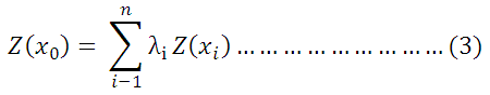
When n is the number of neighbouring samples z (x_i) and λ_i are weights applied to each x (x_i). 

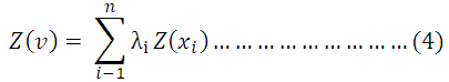
 (2) Block Kriging

In block kriging, a value for an area or block with its centre at x_o is estimated rather than values at points as in punctual kriging.  The kriged value of property z for any block v is a weighted average of the observed values x₁ in the neighbourhood of the block i.e.

(3) Co-kriging

The co-regionalization of two variables z₁ and z₂ is summarized by the cross-semi variogram.

           

Co-kriging has been applied only to point estimation of soil properties. 

(4) Universal Kriging

Universal Kriging was designed to permit kriging in the presence of trends in the sample data i.e.            

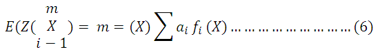
E(Z(x)) is the expected value of the sample data, m (x) is the trend, f_i are the terms in the polynomial and are the co-efficient of the polynomial that describes the trend.