System Engineering 3(3+0)

LESSON 3. Graphical Method II - Special Cases

Example:

Maximize z = x₁ + 2x₂

subject to

x₁ ≤ 80
x₂ ≤ 60
5x₁ + 6x₂ ≤ 600
x₁ + 2x₂ ≤ 160

x₁, x₂ ≥ 0.

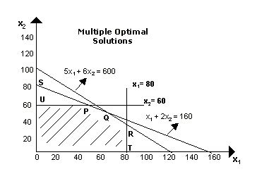
In the above figure, there is no unique outer most corner cut by the objective function line. All points from P to Q lying on line PQ represent optimal solutions and all these will give the same optimal value (maximum profit) of Rs. 160. This is indicated by the fact that both the points P with co-ordinates (40, 60) and Q with co-ordinates (60, 50) are on the line x₁ + 2x₂ = 160. Thus, every point on the line PQ maximizes the value of the objective function and the problem has multiple solutions.

3.2. Infeasible Problem

In some cases, there is no feasible solution area, i.e., there are no points that satisfy all constraints of the problem. An infeasible LP problem with two decision variables can be identified through its graph. For example, let us consider the following linear programming problem.

Minimize z = 200x₁ + 300x₂

subject to

2x₁ + 3x₂ ≥ 1200
x₁ + x₂ ≤  400
2x₁ + 1.5x₂ ≥  900

x₁, x₂ ≥ 0

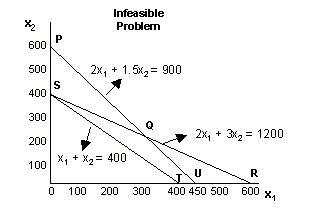
The region located on the right of PQR includes all solutions, which satisfy the first and the third constraints. The region located on the left of ST includes all solutions, which satisfy the second constraint. Thus, the problem is infeasible because there is no set of points that satisfy all the three constraints.

3.3. Unbounded Solutions

It is a solution whose objective function is infinite. If the feasible region is unbounded then one or more decision variables will increase indefinitely without violating feasibility, and the value of the objective function can be made arbitrarily large. Consider the following model:

Minimize z = 40x₁ + 60x₂

subject to

                             2x₁+ x₂ ≥ 70
                               x₁ + x₂ ≥ 40
                               x₁ + 3x₂ ≥ 90

                               x₁, x₂ ≥ 0

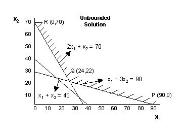
The point (x₁, x₂) must be somewhere in the solution space as shown in the figure by shaded portion.

The three extreme points (corner points) in the finite plane are:
P = (90, 0); Q = (24, 22) and R = (0, 70)  The values of the objective function at these extreme points are: Z(P) = 3600, Z(Q) = 2280 and Z(R) = 4200.

In this case, no maximum of the objective function exists because the region has no boundary for increasing values of x₁ and x₂. Thus, it is not possible to maximize the objective function in this case and the solution is unbounded.

Note:

Although it is possible to construct linear programming problems with unbounded solutions numerically, but no linear programming problem formulated from a real life situation can have unbounded solution.

Limitations of Linear Programming

• Linearity of relations: A primary requirement of linear programming is that the objective function and every constraint must be linear. However, in real life situations, several business and industrial problems are nonlinear in nature.

• Single objective: Linear programming takes into account a single objective only, i.e., profit maximization or cost minimization. However, in today's dynamic business environment, there is no single universal objective for all organizations.

• Certainty: Linear Programming assumes that the values of co-efficient of decision variables are known with certainty.

•  Due to this restrictive assumption, linear programming cannot be applied to a wide variety of problems where values of the coefficients are probabilistic.

• Constant parameters: Parameters appearing in LP are assumed to be constant, but in practical situations it is not so.

• Divisibility: In linear programming, the decision variables are allowed to take non-negative integer as well as fractional values. However, we quite often face situations where the planning models contain integer valued variables. For instance, trucks in a fleet, generators in a powerhouse, pieces of equipment, investment alternatives and there are a myriad of other examples. Rounding off the solution to the nearest integer will not yield an optimal solution. In such cases, linear programming techniques cannot be used.

Summary:

This chapter initiated your study of linear models. Linear programming is a fascinating topic in operations research with wide applications in various problems of management, economics, finance, marketing, transportation and decision making pertaining to the operations of virtually any private or public organization. Unquestionably, linear programming techniques are among the most commercially successful applications of operations research.
In this chapter, you learned how to formulate a linear programming problem, and then we discussed the graphical method of solving an LPP with two decision variables.