System Engineering 3(3+0)

LESSON 1. Simplex Method

1.2 Basic Definitions:

Slack Variable:

It is a variable that is added to the left-hand side of a less than or equal to type constraint to convert the constraint into an equality. In economic terms, slack variables represent left-over or unused capacity.

Specifically:

                  a_i1x₁ + a_i2x₂ + a_i3x₃ + .........+ a_inx_n ≤  b_i

can be written as
              a_i1x₁ + a_i2x₂ + a_i3x₃ + .........+ a_inx_n + s_i = b_i     
 Where i = 1, 2, ..., m

Surplus variable:

It is a variable subtracted from the left-hand side of a greater than or equal to type constraint to convert the constraint into equality. It is also known as negative slack variable. In economic terms, surplus variables represent over fulfillment of the requirement.

Specifically:
                  a_i1x₁ + a_i2x₂ + a_i3x₃ + .........+ a_inx_n ≥ b_i

can be written as
             a_i1x₁ + a_i2x₂ + a_i3x₃ + .........+ a_inx_n - s_i = b_i

Where i = 1, 2, ..., m

Artificial variable:

It is a non negative variable introduced to facilitate the computation of an initial basic feasible solution. In other words, a variable added to the left-hand side of a greater than or equal to type constraint to convert the constraint into equality is called an artificial variable.

1.3 Canonical Form:

The general formulation of L.P.P can always be put in the following form:

Maximize z = c₁x₁ + c₂x₂ +……c_nx_n subject to the constraints

a_i1x₁ + a_i2x₂ + a_i3x₃ + .........+ a_inx_n ≤ b_i,      i =1,2,3,....m

x₁,x₂,x₃,....x_n ≥ 0

by making use of some elementary transformations. This form of L.P.P. is called the canonical form of L.P.P.

1.4 Characteristic of Canonical form:

(i) The objective function is of the maximization type

Minimization of f(x) = -Maximization (-f(x))

If we have the objective function as min z then change that as min z = -Max (-z ).

(ii) All the constraints are of the “≤ “type, except for the non-negative restriction

If we have an inequality of “≥” type, multiply both sides by -1. if the constraints is an equation say

                     a_i1x₁ + a_i2x₂+………a_inx_n = b_i

write it as

                 a_i1x₁ + a_i2x₂+………a_inx_n≤ b_i   and

                 a_i1x₁ + a_i2x₂+………a_inx_n ≥ b_i  (or -a_i1x₁ - a_i2x₂-………-a_inx_n ≤ - b_i)

(iii) All the variables are non-negative

If a variable is unrestricted in sign ((i.e.) positive, negative or zero) then replace that variable by difference between two non-negative variables. If x_j is unrestricted in sign replace x_j by x_j = where both and  are both non-negative.

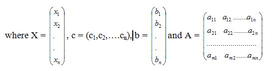
 Matrix Notation of Canonical form:

              In matrix notation the canonical form of L.P.P can be expressed as:

                        Maximize or Minimize z = cx               (Objective Function)

Subject to the constraints:                (Constraints)

                                 AX ≤ b, X ≥ 0              (Non-negative restrictions)

1.5 Standard Form:

The general formulation of L.P.P can always be put in the following form:

Maximize z = c₁x₁ + c₂x₂ +……c_nx_n subject to the constraints

a_i1x₁ + a_i2x₂ + a_i3x₃ + .........+ a_inx_n = b_i,      i =1,2,3,....m

x₁,x₂,x₃,....x_n ≥ 0

is known as in Standard form.

1.6 Characteristic of Standard form:

(i) The objective function is of the maximization type.

(ii) All the constraints are expressed in the form of equations except for the non-negative constraints.

      If the constraints are of “≤” type add the slack variable to the left hand side and if the constraints are of “≥” type subtract surplus variable to the left hand side.

(iii)  The right hand side of each constraint equation is of non-negative.

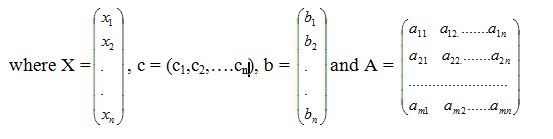
1.7 Matrix Notation of Standard form:  

In matrix notation the Standard form of L.P.P can be expressed as:

                        Maximize or Minimize z = cx               (Objective Function)

       Subject to the constraints:                (Constraints)

                                 AX = b, X ≥ 0              (Non-negative restrictions)

Basic Solution, Basic and Non- basic variable:

Given a system of m linear equations with n variables (m < n). The solution obtained by setting (n – m) variables equal to zero and solving for the remaining m variables is called a basic solution.

The m variables are called basic variables and they form the basic solution. The n-m variables which are put to zero are called as non-basic variables.

Degenerate basic solution:

A basic solution is said to be a degenerate basic solution if one or more of the basic variables are zero.

Basic Feasible solution:

A feasible solution which is also basic is called a Basic Feasible solution.

 1.8 ALGORITHM OF SIMPLEX METHOD

 Assuming the existence of an initial basic feasible solution, an optimal solution to any L.P.P by simplex method is found as follows:

 Step 1: Check whether the objective function is to be maximized or minimized. If it is to be minimized, then convert it into a problem of maximization, by

Minimize Z = -Maximize (-Z)

Step 2: Check whether all b_i’s are positive. If any of the b_i’s is negative, multiply both sides of that constraint by -1 so as to make its right hand side positive.

Step 3: By introducing slack / surplus variables, convert the inequality constraints into equations and express the given L.P.P into its standard form.

Step 4: Find an initial basic feasible solution and express the above information conveniently in the following simplex table.

 

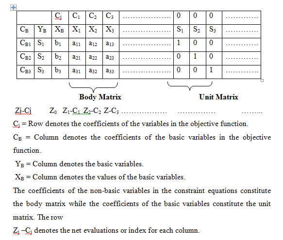
Step 5: Compute the net evaluations Z_j –C_j (j= 1,2,3…..n) by using the relation

Z_j –C_j = C_Ba_j- C_j

Examine the sign of Z_j –C_j

a)     If all Z_j –C_j ≥ 0 then the current basic solution X_B is optimal.

b)    If atleast  Z_j –C_j < 0 then the current basic solution X_B is not optimal, go to next step.

 Step 6: (To find the entering variable)

The entering variable is the non-basic variable corresponding to the most negative value Z_j –C_j. Let it be x_r for some j = r. The entering variable column is known at the bottom. If more than one variable has the same most negative Z_j –C_j, any of these variables may be selected arbitrarily as the entering variable.

 Step 7: (To find the leaving variable)

Compute the ratio;

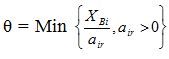
(i.e) the ratio between the solution column and the entering variable column by considering only the positive denominators.

a)     If all a_ir ≤ 0, then there is an unbounded solution to the given L.P.P.

b)    If all a_ir > 0, then the leaving variable is the basic variable corresponding to the minimum ratio θ. If,

  

then the basic variable x_k leaves the basis. The leaving variable row is called the key row or pivot row or pivot equation and the element at the intersection of the pivot column and pivot row is called the pivot element or key element or leading element.

Step 8:

Drop the leaving variable and introduce the entering variable along with its associated value under C_B column. Convert the pivot element to unity by dividing the pivot equation by the pivot element and all other elements in its column to zero by making use of 

•  New pivot equation = old pivot equation / pivot element

•  New equation (all other rows including Z_j –C_j row)

    New equation = (Corresponding element) X New pivot equation

Step 9: Go to step 5 and repeat the procedure until either an optimum solution is obtained or there is an indication of an unbounded solution. 

 Example:

Maximize z = 3x₁ + 2x₂

Subject to

-x₁ + 2x₂ ≤ 4
3x₁ + 2x₂ ≤  14
   x₁ – x₂ ≤  3

x₁, x₂ ≥ 0

Solution:

First, convert every inequality constraints in the LPP into an equality constraint, so that the problem can be written in a standard from. This can be accomplished by adding a slack variable to each constraint. Slack variables are always added to the less than type constraints.

 Converting inequalities to equalities

-x₁ + 2x₂ + x₃ = 4
3x₁ + 2x₂ + x₄ = 14
x₁ – x₂ + x₅ = 3
x₁, x₂, x₃, x₄, x₅ ≥  0

where x₃, x₄ and x₅ are slack variables.

Since slack variables represent unused resources, their contribution in the objective function is zero. Including these slack variables in the objective function, we get

Maximize z = 3x₁ + 2x₂ + 0x₃ + 0x₄ + 0x₅

Initial basic feasible solution

Now we assume that nothing can be produced. Therefore, the values of the decision variables are zero. x₁ = 0, x₂ = 0, z = 0

When we are not producing anything, obviously we are left with unused capacity
x₃ = 4, x₄ = 14, x₅ =

We note that the current solution has three variables (slack variables x₃, x₄ and x₅) with non-zero solution values and two variables (decision variables x₁ and x₂) with zero values. Variables with non-zero values are called basic variables. Variables with zero values are called non-basic variables.

Iteration 1:

	cj	3	2	0	0	0
cB	Basic variables B	x1	x2	x3	x4	x5	Solution values b (=XB)
0	x3	-1	2	1	0	0	4
0	x4	3	2	0	1	0	14
0	x5	1	-1	0	0	1	3
zj-cj		-3	-2	0	0	0

 

a₁₁ = -1, a₁₂ = 2, a₁₃ = 1, a₁₄ = 0, a₁₅ = 0, b₁ = 4
a₂₁ = 3, a₂₂ = 2, a₂₃ = 0, a₂₄ = 1, a₂₅ = 0, b₂ = 14
a₃₁= 1, a₃₂ = -1, a₃₃ = 0, a₃₄ = 0, a₃₅ = 1, b₃ = 3

Calculating values for the index row (z_j – c_j)

z₁ – c₁ = (0 × (-1) + 0 × 3 + 0 × 1) - 3 = -3
z₂ – c₂ = (0 × 2 + 0 × 2 + 0 × (-1)) - 2 = -2
z₃ – c₃ = (0 × 1 + 0 × 0 + 0× 0) - 0 = 0
z₄ – c₄ = (0 × 0 + 0 × 1 + 0 × 0) - 0 = 0
z₅ – c₅ = (0 × 0 + 0×0 + 0×1) – 0 = 0

Choose the smallest negative value from z_j – c_j (i.e., – 3). So column under x₁ is the key column.
Now find out the minimum positive value
Minimum (14/3, 3/1) = 3
So row x₅ is the key row.
Here, the pivot (key) element = 1 (the value at the point of intersection).
Therefore, x₅ departs and x₁ enters.

We obtain the elements of the next table using the following rules:

1. If the values of z_j – c_j are positive, the inclusion of any basic variable will not increase the value of the objective function. Hence, the present solution maximizes the objective function. If there are more than one negative values, we choose the variable as a basic variable corresponding to which the value of z_j – c_j is least (most negative) as this will maximize the profit.

2. The numbers in the replacing row may be obtained by dividing the key row elements by the pivot element and the numbers in the other two rows may be calculated by using the formula:

   

Calculating values for Iteration 2

 x₃ row

a₁₁ = -1 – 1 × ((-1)/1) = 0
a₁₂ = 2 – (-1) × ((-1)/1) = 1
a₁₃ = 1 – 0 × ((-1)/1) = 1
a₁₄ = 0 – 0 × ((-1)/1) = 0
a₁₅ = 0 – 1 × ((-1)/1) = 1
b₁ = 4 – 3 × ((-1)/1) = 7

x₄ row

a₂₁ = 3 – 1× (3/1) = 0
a₂₂ = 2 – (-1) × (3/1) = 5
a₂₃ = 0 – 0 × (3/1) = 0
a₂₄ = 1 – 0 × (3/1) = 1
a₂₅ = 0 – 1 × (3/1) = -3
b₂ = 14 – 3 × (3/1) = 5

x₁ row

a₃₁ = 1/1 = 1
a₃₂ = -1/1 = -1
a₃₃ = 0/1 = 0
a₃₄ = 0/1 = 0
a₃₅ = 1/1 = 1
b₃ = 3/1 = 3

Iteration 2:

	cj	3	2	0	0	0
cB	Basic variables B	x1	x2	x3	x4	x5	Solution values b (= XB)
0	x3	0	1	1	0	1	7
0	x4	0	5	0	1	-3	5
3	x1	1	-1	0	0	1	3
zj-cj		0	-5	0	0	3

 

Calculating values for the index row (z_j – c_j)

z₁ – c₁ = (0 × 0 + 0 × 0 + 3 × 1) - 3 = 0
z₂ – c₂ = (0 × 1 + 0 × 5 + 3 × (-1)) – 2 = -5
z₃ – c₃ = (0 × 1 + 0 × 0 + 3 × 0) - 0 = 0
z₄ – c₄ = (0 × 0 + 0 × 1 + 3 × 0) - 0 = 0
z₅ – c₅ = (0 × 1 + 0 × (-3) + 3 × 1) – 0 = 3

Key column = x₂ column
Minimum (7/1, 5/5) = 1
Key row = x₄ row
Pivot element = 5
x₄ departs and x₂ enters.

Calculating values for table 3

x₃ row

a₁₁ = 0 – 0× (1/5) = 0
a₁₂ = 1 – 5 × (1/5) = 0
a₁₃ = 1 – 0 × (1/5) = 1
a₁₄ = 0 – 1× (1/5) = -1/5
a₁₅ = 1 – (-3) × (1/5) = 8/5
b₁ = 7 – 5 × (1/5) = 6

x₂ row

a₂₁ = 0/5 = 0
a₂₂ = 5/5 = 1
a₂₃ = 0/5 = 0
a₂₄ = 1/5
a₂₅ = -3/5
b₂ = 5/5 = 1

x₁ row

a₃₁ = 1 – 0 × (-1/5) = 1
a₃₂ = -1 – 5× (-1/5) = 0
a₃₃ = 0 – 0 × (-1/5) = 0
a₃₄ = 0 – 1 × (-1/5) = 1/5
a₃₅ = 1 – (-3) × (-1/5) = 2/5
b₃ = 3 – 5 × (-1/5) = 4

Note: Don't convert the fractions into decimals, because many fractions cancel out during the process while the conversion into decimals will cause unnecessary complications.

Final iteration:

	cj	3	2	0	0	0
cB	Basic variables B	x1	x2	x3	x4	x5	Solution values b (= XB)
0	x3	0	0	1	-1/5	8/5	6
2	x2	0	1	0	1/5	-3/5	1
3	x1	1	0	0	1/5	2/5	4
zj-cj		0	0	0	1	0

 

Result:

Since all the values of zj – c_j are positive, this is the optimal solution.
x₁ = 4, x₂ = 1
                              Max z = 3 X ₄ + 2 X ₁ = 14.

The largest profit of Rs.14 is obtained, when 1 unit of x₂ and 4 units of x₁ are produced. The above solution also indicates that 6 units are still unutilized, as shown by the slack variable x₃ in the X_B column.

Minimization Case:

 In the previous section, the simplex method was applied to linear programming problems where the objective was to maximize the profit with less than or equal to type constraints. In many cases, however, constraints may of type ≥ or = and the objective may be minimization (e.g., cost, time, etc.). Thus, in such cases, simplex method must be modified to obtain an optimal policy.

Consider the general linear programming problem

Minimize z = c₁x₁ + c₂x₂ + c₃x₃ + .........+ c_nx_n

subject to

a₁₁x₁ + a₁₂x₂ + a₁₃x₃ + .........+ a_1nx_n ≥ b₁
a₂₁x₁ + a₂₂x₂ + a₂₃x₃ + .........+ a_2nx_n≥  b₂
................................................................
   a_m1x₁ + a_m2x₂ + a_m3x₃ + .........+ a_mnx_n≥  b_m
x₁, x₂,....., x_n≥ 0

Changing the sense of the optimization

             Any linear minimization problem can be viewed as an equivalent linear maximization problem, and vice versa.

Min. z = c₁x₁ + c₂x₂ + c₃x₃ + .........+ c_nx_n

It can be written as

Max. z = - (c₁x₁ + c₂x₂ + c₃x₃ + .........+ c_nx_n)

Converting inequalities to equalities

             Introducing surplus variables (negative slack variables) to convert inequalities to equalities

a₁₁x₁ + a₁₂x₂ + a₁₃x₃ + .........+ a_1nx_n - s₁ = b₁
a₂₁x₁ + a₂₂x₂ + a₂₃x₃ + .........+ a_2nx_n - s₂ = b₂

….................................................................
    a_m1x₁ + a_m2x₂ + a_m3x₃ + .........+ a_mnx_n - s_m = b_m
x₁, x₂,....., x_n ≥ 0
s₁, s₂,....., s_m ≥ 0

An initial basic feasible solution is obtained by setting x₁ = x₂ =........ = x_n = 0

-s₁ = b₁ or s₁ = -b₁
-s₂ = b₂ or s₂ = -b₂
 ..............................
  -s_m = b_m or s_m = -b_m

which is not feasible because it violates the non-negativity stipulation, (i.e., s₁≥  0). Therefore, we need artificial variables.

After introducing artificial variables, the set of constraints can be written as

a₁₁x₁ + a₁₂x₂ + a₁₃x₃ + .........+ a_1nx_n - s₁ + A₁ = b₁
a₂₁x₁ + a₂₂x₂ + a₂₃x₃ + .........+ a_2nx_n - s₂ + A₂ = b₂
..............................................................................
a_m1x₁ + a_m2x₂ + a_m3x₃ + .........+ a_mnx_n - s_m + A_m = b_m

x₁, x₂,....., x_n ≥ 0
s₁, s₂,....., s_m ≥ 0
A₁, A₂,....., A_m ≥ 0

Now, an initial basic feasible solution can be obtained by setting all the decision and surplus variables to zero. Thus, an initial basic feasible solution to LPP is
       A₁ = b₁ , A₂ = b₂, ....., A_m = b_m

Now to obtain an optimal solution, we must drive out the artificial variables. The two methods to solve linear programming problems in such cases are:

• Two Phase method

• Big-M- method

LIMITATIONS OF SIMPLEX METHOD:

• Inability to deal with multiple objectives.

• Inability to handle problems with integer variables.

• Solution methods to LP problems with integer or Boolean variables are still far less efficient than those which include continuous variables only.