System Engineering 3(3+0)

LESSON 2. TRANSPORTATION PROBLEMS

1. Least Time Transportation Problems

There are some transportation problems where the objective is to minimize time rather than transportation cost. Such problems are usually encountered in hospital management, military services, fire services, etc. where the speed of delivery or time of supply is more important than the transportation cost.

Now, while solving problems where the objective is to minimize time for each route, the cost per unit is replaced by the time required to ship the quantity x_ij from origin i to destination j, where i=1,2,3, ….. ,m and j= 1,2,3, ….. ,n. The corresponding transportation matrix is given below.

 

                                      

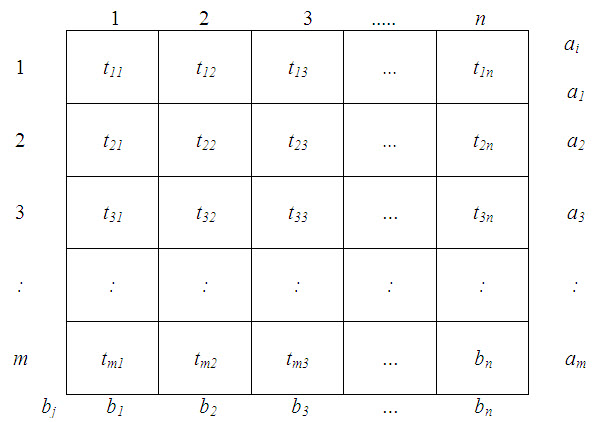
                    _{m               n}                     

 and             Σ  a_i  =    Σ  b_j

                  ^{i =1                 j = 1}    

Note that the time of shipment is independent of the number of units shipped. Also since shipments from origins to destinations can be done at the same time on different routes, the shipment time of the total plan is not the sum total of the times of the individual routes. In fact, the shipment of a feasible plan will be complete. Such problems, therefore, require a different solution procedure.

Let,  T_k be the largest time associated with k^th feasible plan. Our objective is, therefore, to find out a plan for which T_k is minimum of all values of k. The procedure for getting minimum T_k consists of the following steps:

Step I: Find an initial basic feasible solution. This is obtained by using the same method as for the normal transportation technique.

Step II: Find T_k corresponding to the current feasible solution and cross out all the non-basic cells for which t_ij ≥T_k.

Step III: Draw a closed path (as in the normal transportation technique) for the basic variable associated with T_k such that when the values at the corner elements are shifted around, this basic variable reduces to zero and no variable becomes negative. This procedure ends if no such closed path can be traced out, otherwise repeat step II.

 1.1.Post optimality analysis in transportation

The transportation models studied above will normally be valid for a limited period only. In actual practice, the resource capacities and/or destination requirements may vary with time. Likewise, there may be some changes in the transportation cost. Such changes may affect the optimal allocation and the associated transportation cost. One way to study the effect of these changes is to solve the problem a new. Many a times, however, it may not be necessary to do so and the new optimal solution may be obtained by simply incorporating the changes in the current optimal solution, seeing the effects of these changes and carrying out iterations if required. 

1.2. Changes in transportation costs

An increase in the costs of empty cells will not change the current optimal solutions as the current cost itself is too high, that is why there have been no allocations in these cells.

However, a reduction in costs of empty cells or an increase in costs of allocated cells is likely to change the transportation schedule. In this case the problem is re-considered with the current optimal solution. New values of u_i and v_j numbers are computed and evaluations of the empty cells are determined. If they are all non-negative, the current solution still remains optimal. If not, a new solution is obtained which is then tested for optimality.

 1.3. The trans-shipment problem

The transportation problem assumes that direct routes exist from each source to each destination. However, there are situations in which units may be shipped from one source to another or to other destinations before reaching their final destination. This is called a trans-shipment problem. For example, movement of material involving two different modes of transport – road and railways or between stations connected by broad gauge to metre gauge lines will necessarily require transshipment. For the purpose of transshipment the distinction between a source and destination is dropped so that a transportation problem with m sources n destinations gives rise to a transshipment problem will involve [(m+n)+(m+n)–1] or   [2m+2n–1] basic variables and if we omit the variables appearing in the (m+n) diagonal cells, we are left with [m+n–1]  basic variables.

In the trans-shipment problem, as each source or destination is a potential point of supply as well as demand, the total supply, say of N units, is added to the actual supply of each source, as well as to the actual demand at each destination. Also the ‘demand’ at each source and ‘supply’ at each destination are set equal to N.

Therefore, we may assume the supply and demand of each location to be fictitious one. These qualities (N) may be regarded as buffer stocks and each of these buffer stocks should at least be equal to the total supply/demand in the given problem.

The given trans-shipment problem can, therefore, be regarded as the extended transportation problem and can hence be solved by the transportation technique. In the final solution, units transported from a point to itself i.e., in diagonal cells are ignored as they do not have any physical meanings as there is no transportation involved.

 1.4. Dual of the transportation problem

We know any linear programming problem has its dual. Since the transportation problem is a special type of linear programming problem, it also has its dual with usual interpretations and applications. To illustrate let us consider example along with the transportation cost table. The mathematical model (Primal) for this problem is rewritten below:

Minimize, Z = 2x₁₁ + 3x₁₂ + 11x₁₃ + 7x₁₄ +  x₂₁ + 0x₂₂ + 2x₁₁ + 6x₂₃ + x₂₄ + 5x₃₁ + 8x₃₂ + 15x₃₃ + 9x₃₄ ,

Subject to constraints

 x₁₁ + x₁₂ + x₁₃ + x₁₄ =6,

 x₂₁ + x₂₂ + x₂₃ + x₂₄ =1,

 x₃₁ + x₃₂ + x₃₃ + x₃₄ =10,

 x₁₁ + x₂₁ + x₃₁=7,

 x₂₁ + x₂₂ + x₃₃ =5,

 x₁₃ + x₂₃ + x₃₃=3,

 x₁₄ + x₂₄ + x₃₄=2,

 where, x_ij ≥0; i =1,2,3; j = 1,2,3,4.

 Now the dual of this linear problem can be written as,

 maximize

 Z’ = 6u₁+u₂ +10 u₃+7v₁+5v₂+3v₃+2v₄,

 Subject to

             u₁+v₁≤ 2,

             u₁+v₂≤3,

 u₁+v₃≤11,

 u₁+v₄≤ 7,

 u₂+v₁≤ 1,

 u₂+v₂≤ 0,

 u₂+v₃≤ 6,

 u₂+v₄≤ 1,

 u₃+v₁≤ 5,

 u₃+v₂≤ 8,

 u₃+v₃≤15, 

u₃+v₄≤9, 

where the dual variables u_i and v_j are unrestricted in sign,

 i =1,2,3 ;          j=1,2,3,4.

 1.5. Interpretation of the dual 

1. The dual variables u_i and v_j are the row numbers and column numbers respectively in table, used in solving the problem by the modified distribution method. In dual, u_i may be interpreted as the value of the product, free on board, at the i^th origin and, therefore, may be called location rent and v_j can be interpreted as its value (delivered) at the j^th  destination and, therefore, may be termed market prize. Hence Z’ which represents the sum of these two factors is to be maximized. The constraints of the dual indicate that to allocate in a cell, the transportation cost in that cell should not be more than the sum of these two factors for that cell.
2. We know that in case of linear programming, the final (optimal) simplex table also represents the optimal solution of the dual without actually solving it. Likewise, the optimal (final) transportation table of the primal represents the optimal solution of the associated dual. For the problem under consideration, the optimal dual solution as given by table.

 u₁=1,  u₂=- 4, u₃=5, v₁= 0, v₂=2, v₃=10, v₄=4 .
 value of  
 Z’_max  =  Rs. 100 [ 6 x 1 – 1 x 4 + 10 x 5 + 7 x 0 +5 x 2 + 3  x 10 + 2 x 4 ] 
            = Rs. 100 [ 6 – 4 + 50 + 0 + 10 + 30 + 8 ] 
            = Rs. 10,000 , which is same as Z’ _min .

2. Minimization  of Transportation Cost Using Distribution Linear Programming

If the problem can be formulated (modeled) as one of minimizing some given cost, such as transportation expense, the methods of distribution linear programming are useful techniques for minimizing the cost function subject to supply and demand constraints.

Distribution linear programming methods are widely used for minimizing transportation costs and are indeed useful in numerous other maximization or minimization situations, such as maximizing revenue available from various alternative locations, minimizing unit production costs, and minimizing materials handling costs. The demand requirements and supply availabilities (demand-supply constraints) are typically formulated in a rectangular arrangement (matrix) with the transported amounts (cell loadings) being governed by the cost or profit for the particular supply- demand route. Several methods of obtaining initial and final solutions have been developed, some of which include the following.

         I. Initial solutions

1. North west corner method

2. Minimum matrix method (minimum cost)

3. Vogel’s approximation method

       II. Optimal solutions

1. Stepping- stone method

2. Modified distribution method (MODI)

The following example will illustrate the use of an initial allocation via the North West corner method and a final solution via the stepping- stone method. These are not usually the most expedient methods to follow when the problem has any degree of complexity, but they have intuitive value and quickly convey the basic methodology. An optional problem in the solved problem section at the end of this chapter illustrates the use of the minimum cost method. 

The solution procedure necessitates that only unused transportation paths (vacant cells) be evaluated, and there is only one available pattern of moves to evaluate each vacant cell. This is because moves are restricted to occupied cells. Every time a vacant cell is filled, one previously occupied cell must become vacant. The initial (and continuing) number of entries is always maintained at R+C-1, that is, number of rows plus number of columns minus one. When a move happens to cause fewer entries (for example, when two cells become vacant at the same time but only one is filled), a “zero” entry must be retained in one of the cells to avoid what is termed a “degeneracy” situation. The zero entry should be assigned to an independent cell, that is, to one that cannot be reached by a closed path involving only filled cells. The cell with the zero entry is then considered to be an occupied and potentially usable cell.

A second potentially troublesome situation may arise when supply and demand are unequal. In this situation a “dummy” supply plant or absorption location can be created either to produce the additional needed supply or to absorb the excess supply.

If demand > supply: create a dummy supply and assign zero transportation cost to it so excess demand is satisfied.

If supply> demand: create a dummy demand and assign zero transportation cost to it so excess supply is absorbed. 

• This corresponds to a fundamental linear programming rule which holds that the number of variables in solution must equal the number of constraints that are binding.

Problem No.1:

Obtain an initial basic feasible solution to the following distribution of products to various destinations from the sources. 

Sources, b	Destinations, a				Supply, Sbj
	a1	a2	a3	a4
b1	11	13	17	14	250
b2	16	18	14	10	300
b3	21	24	13	10	400
Demand, Sai	200	225	275	250

 

Solution : Since, Sa_i=Sb_j=950, there exists a feasible solution to the transportation problem.  The initial feasible solution can be obtained as given below.

North West Corner Rule (NWC)

Step 1: Starting with the cell at the upper left (north-west) corner of the transportation matrix, allocate as much as possible so that either the capacity of the first row is exhausted or the destination requirement of the first column is satisfied. i.e x₁₁=min(a₁,b₁).

Step 2: If b₁> a₁, the move down vertically to the second row and make the second allocation of magnitude x₁₂ = min (a_2,b_1- x₁₁) in the cell (2,1).

If b₁<a₁, then move right horizontally to the second column and make the second allocation of magnitude x₁₂ = min (a_{1 -} x_11,b₂) in the cell (1,2).

If, b₁=a₁, there is a tie for the second allocation of magnitude x₁₂ = min (a_{1 -} a_{1 ,}b₁) = 0 in the cell (1,2),  or x₂₁=min(a_2,b_1- b₁ ) = 0 in the cell (2,1).

Step 3: Repeat steps 1 and 2 moving down towards the lower right corner of the transportation table until all the rim requirements are satisfied.

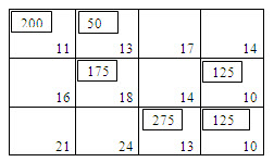
The transportation table of the given problem has 12 cells.  Following north-west corner rule, the first allocation is made to the cell (1, 1), the magnitude being x₁₁ = min. (250, 200) = 200.  The second allocation is made to the cell (1, 2) and the magnitude of the allocation is given by,

x₁₂ = min. (250 – 200, 50) = 50.

The third allocation is made in the cell (2, 2), the magnitude being x₂₂= min. (300, 225-50)=175. In the cell (2, 3) is given by x₂₃=min. (300 – 175, 275) = 125.  The fifth allocation is made in the cell (3, 3), the magnitude being  x₃₄ = min. (400-150, 250)=250.  Hence an initial basic feasible solution to the given transportation problem is obtained and given below.

  

 

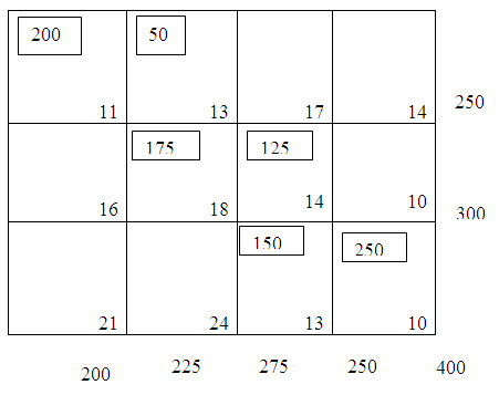
Table – 1

The transportation cost according to the above route is given by,

            z = (200x11) + (50x13) + (175x18) + (125x14) + (150x13) + (20x10)

               = Rs.12,200.

Least cost or Matrix Minima method

Step 1 : Determine the smallest cost in the cost matrix of the transportation table. Let it be C_ij. Allocate x_ij = min (a_i, b_j) in the cell (i,j).

Step 2 : If,  x_j = a_i, cross off the i^th row of the transportation table and decrease b_j by a_i. Go to step3.

            If  x_ij = b_j, cross off the j^th column of the transportation table and decrease a_i by b_j. Go to step3.

If  x_j = a_i = b_j,  cross off  either the i^th row or j^th column but not both.

Step 3 : Repeat steps1 and 2 for the resulting reduced transportation table until all the rim requirements are satisfied. Whenever the minimum cost is not unique, make an arbitrary choice among the minima.

Problem: Obtain an initial basic feasible solution to the following distribution of products to various destinations from the sources as given in Problem No.1.

 

Sources, b	Destinations, a				Supply, Sbj
	a1	a2	a3	a4
b1	11	13	17	14	250
b2	16	18	14	10	300
b3	21	24	13	10	400
Demand, Sai	200	225	275	250

 

Solution : Since, Sa_i=Sb_j=950, there exists a feasible solution to the transportation problem.  The initial feasible solution can be obtained as given below following Least-Cost Method.

Following the least cost method, the first allocation is made in the cell (3,4), the magnitude being x₃₄ = min. (400, 250)=250.  This satisfies the requirement at a₄ and thus we cross off the fourth column from the table.  The second allocation is made in the cell (1, 1) of magnitude x₁₁ = min. (250, 200) = 200 which satisfied the required at a₁ and therefore, we cross off the first column from the table.  This yields table 2.

 

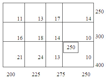
Table – 1

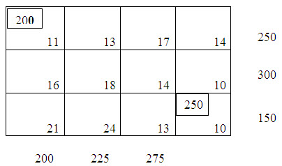
Table – 2

Now there is a tie for third allocation.  We choose arbitrarily the cell (1, 2) and allocate x₁₂= min. (50, 225) = 50.  Cross off the first row.  Fourth allocation is made in the cell (3, 3) with magnitude x₃₃= min.(150, 275)=150.  After crossing off the third row, it  results in table 3.

  

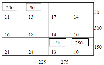
Table – 3

 

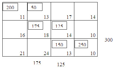
Table – 4

Fifth allocation is made to the cell (2, 3) of magnitude x₂₃=min. (300, 125) = 125 and the sixth allocation is given by x₂₂=min (175, 175) = 175.

 

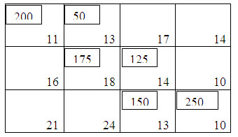
                                                                      Table - 5

 Thus we get the initial basic feasible solution as displayed in table 5.  The transportation cost according to the above route is given by,

 z = (200x11) + (50x13) + (175x18) + (125x14) + (150x13) + (250x10) = Rs.12,200.

 

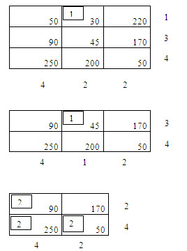
The Row Minima Method

Step 1 : The smallest cost in the first row of the transportation table is determined. Let it be C_ij. Allocate the maximum feasible  x_ij=min (a₁,b_j) in the cell (1,j).

Step 2: If  x_1j=a₁, cross off the 1^st  row of the transportation table and move down to the second row. If  x_1j=b_j, cross off the j^th column of the transportation table and reconsider the first row with the remaining availability.

If  x_1j=a₁=b_j,  cross off  the 1^st column and make the second allocation x_1k=0 in the cell (1,k) with C_1k being the new minimum cost in the first row. Cross of the first row and move down to the second row.

Step 3: Repeat steps1 and 2 for the resulting reduced transportation table until all the rim requirements are satisfied.

Problem:

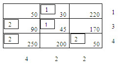
Determine an initial basic feasible solution to the following transportation problem following row minima method.

Sources	Destimation			Supply, Units
	A	B	C
I	50	30	220	1
II	90	45	170	3
III	250	200	50	4
Requirements	4	2	2

Solution:

The Column Minima Method 

Step 1: Determine the smallest cost in the first column of the transportation table. Let it be C_i1. Allocate the maximum feasible units to x_i1=min(a_i,b₁) in the cell (i,1). 

Step 2: If  x_i1=a_i, cross off the i^th row of the transportation table and reconsider the first column with the remaining availability. 

If,  x_i1=b₁, cross off the i^th column and move towards right to the second column.

If,  x_i1=a_i=b₁,  cross off  the i_th row and make the second allocation x_k1=0 in the cell (k,1) with C_k1 being the new minimum cost in the first column. Cross of the first column and move down to the second column. 

Step 3: Repeat steps1 and 2 for the resulting reduced transportation table until all the rim requirements are satisfied.

Problem:

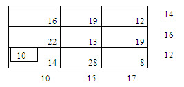
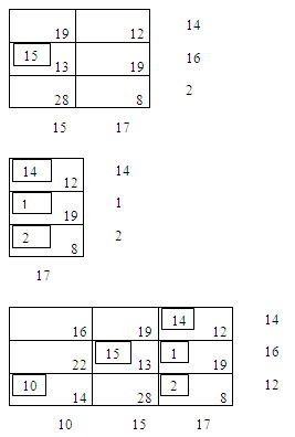
Determine an initial basic feasible solution to the following  transportation problem using column minima method.

Sources	Destination			Supply, Units
	A	B	C
I	16	19	12	14
II	22	13	19	16
III	14	28	8	12
Requirements	10	15	17

 

Solution :

 

Vogels approximation method (VAM or penalty method):

Step 1: Calculate the penalties by taking differences between the minimum and next to minimum unit transportation costs in each row and each column.

Step 2: Circle the largest row difference or column difference. In the event of a tie, choose either.

Step 3: Allocate as much as possible in the lowest cost cell of the row(or column) having a circled row (or column) difference.

Step 4: In case the allocation is made fully to a row (or column) , ignore that row(or column)  for further consideration, by crossing it.

Step 5: Revise the differences again and cross out the earlier figures. Go to step2.

Step 6: Continue the procedure until all rows and columns have been crossed out, i.e distribution is complete.

Problem

Obtain an initial basic feasible solution to the following transportation.
                         

Sources, b	Destinations, a				Supply, Sbj
	a1	a2	a3	a4
b1	11	13	17	14	250
b2	16	18	14	10	300
b3	21	24	13	10	400
Demand, Sai	200	225	275	250

 

Solution: Since, Sa_i=Sb_j=950, there exists a feasible solution to the transportation problem.  The initial feasible solution can be obtained as given below. 

Following the Vogels approximation method, the differences between the smallest and next to smallest costs in each row and each column are computed and displayed inside the parenthesis against the respective rows and columns.  The largest of these differences is (5) and is associated with the first column of the transportation table.

Since the minimum cost in the first column is c₁₁= 11, allocate x11=min. (250, 200)=200 in the cell (1,1).  This exhausts the requirement of the first column and, therefore, cross off the first column.  The row and column differences are now computed for the resulting reduced transportation table 1, the largest of these is (5) which is associated with the second column.  Since c₁₂ (=13) is the minimum cost, allocate x₁₂ = min.  (50, 225) = 50.

 

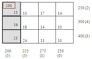
Table – 1

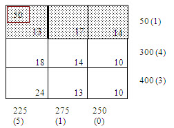
Table – 2

 Thus exhausts the availability of first row and, therefore, we cross off the first row.  Continuing in this manner, the subsequent reduced transportation tables and the differences for the surviving rows and columns are shown in table: 

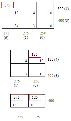
Eventually, the basic feasible solution obtained is shown in the following table: 

The transportation cost according to this route is given by 

z = (200x11) + (50x13) + (175x18) + (125x10) + (275x13) + (125x10) = Rs.12,075