Strength of Material 3(2+1)

LESSON 24. Beam-Column

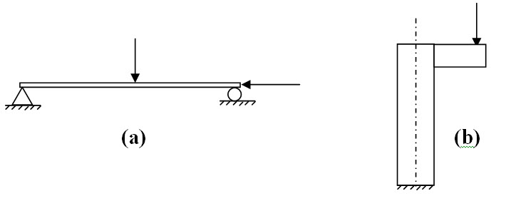
Fig. 24.1.

In this lesson we will derive the governing differential equation for beam-column and illustrate its application in different problems.

24.1 Differential Equation for Beam-Column

Consider a slender member subjected simultaneously to an arbitrary lateral load and an axial load as shown in Figure 24.2a. Free body diagram of an infinitesimal segment dx, in its deformed configuration is shown in Figure

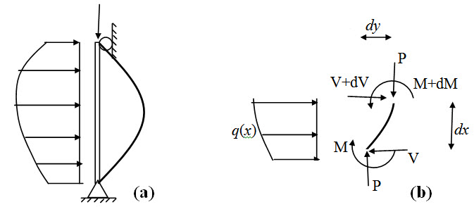
Fig. 24.2.

Applying the static equilibrium conditions,

\[\sum{{F_x}=0}\Rightarrow V + dV - V + q(x)dx\]

\[{{dV} \over {dx}}=-q(x)\]                                     (24.1)

\[\sum {M = 0}\Rightarrow-\left( {M + dM} \right) + M + Vdx + Pdy + qdx{{dx} \over 2}=0\]

\[\Rightarrow-{{dM} \over {dx}} + P{{dy} \over {dx}}=-V\]   [ Neglecting second order term (dx)²]                   (24.2)

Differentiating Equation (24.2) with respect to y,

\[\Rightarrow-{{{d^2}M} \over {d{x^2}}} + {d \over {dx}}\left( {P{{dy} \over {dx}}} \right)=-{{dV} \over {dx}}\]                         (24.3)

From the equation of elastic line, we have,

\[{{{d^2}y} \over {d{x^2}}}=-{M \over {EI}}\]                              (24.4)

Substituting Equations (24.1) and (24.4), Equation (24.3) becomes,

\[{{{d^4}y} \over {d{x^4}}} + {d \over {dx}}\left( {P{{dy} \over {dx}}} \right)=q(x)\]                               (24.5)

Equation (24.5)  is the beam-column governing differential equation.

 Example

Consider a beam colum subjected simultaneously to a transverse load Q at its mid-span and axial compressive force P as shown in Figure 24.3a.

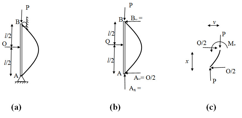
Fig. 24.3.

From Free body diagram of the whole structure (Figure 24.3b), support reactions are,

\[{A_x} = P\]  and   \[{A_y} = {B_y} = Q/2\]

From Free body diagram Figure 24.3c,

\[\sum {{M_x} = 0}\Rightarrow-{M_x} + {Q \over 2}x + Py = 0\]   for  \[0 \le x \le l/2\]                     (24.6)

Substituting equation of elastic line (Equation 24.4) into Equation 24.6, we have,

\[EI{{{d^2}y} \over {d{x^2}}} + {Q \over 2}x + Py = 0\]                                (24.7)

\[\Rightarrow {{{d^2}y} \over {d{x^2}}} + {k^2}y=-{{Qx} \over {2P}}{k^2}\]           \[\left[ {{k^2}={P \over {EI}}} \right]\]             (24.8)

The general solution of the above differential equation,

\[y = {y_h} + {y_p}\]                     (24.8)

Homogeneous solution y_h is,

\[{y_h}=A\cos kx + B\sin kx\]                (24.10)

Particular solution    y_p      is,

\[{y_p}=C + Dx\]                                     (24.11)

Substituting y_p into Equation (24.8),

\[{{{d^2}{y_p}}\over{d{x^2}}}+{k^2}{y_p}=-{{Qx}\over{2P}}{k^2}\]

\[\Rightarrow{k^2}\left({C+Dx}\right)=-{{Qx}\over{2P}}{k^2}\]

\[\Rightarrow C=0\]  and  \[D=-{Q \over {2P}}\]

Therefore,

\[y=A\cos kx + B\sin kx -{{Qx}\over{2P}}\]                                (24.12)

Constants A and B are determined from the following boundary conditions,

y = 0 at x =0 \[\Rightarrow A=0\]

\[{{dy} \over {dx}}=0\] at x = l/2

\[Bk\cos \left( {\frac{{kl}}{2}} \right) - \frac{Q}{{2P}} = 0 \Rightarrow B = \frac{Q}{{2Pk\cos \left( {\frac{{kl}}{2}} \right)}}\]

Therefore,

\[y = \frac{{Q\sin kx}}{{2Pk\cos \left( {\frac{{kl}}{2}} \right)}} - \frac{{Qx}}{{2P}}\]  for \[0 \le x \le l/2\]                         (24.13)

In this case the maximum displacement occurs at the mid-span,

\[{y_{\max }}=\frac{{Q\sin\left({\frac{{kl}}{2}}\right)}}{{2Pk\cos\left({\frac{{kl}}{2}}\right)}}-\frac{{Ql}}{{4P}}=\frac{Q}{{2Pk}}\left[{\tan\left({\frac{{kl}}{2}} \right)-\frac{{kl}}{2}}\right]\]

\[\Rightarrow {y_{\max }}=\frac{{Q{l^3}{k^2}}}{{2Pk{}^3{l^3}}}\left[{\tan\left({\frac{{kl}}{2}}\right) -\frac{{kl}}{2}}\right]\]

\[\Rightarrow {y_{\max }}=\frac{{Q{l^3}}}{{48EI}}\left[{\frac{{3\left({\tan\alpha-\alpha}\right)}}{{{\alpha^3}}}}\right]\]     \[\left[{\alpha=\frac{{kl}}{2}}\right]\]

\[\Rightarrow {y_{\max}}={y_0}\left[{\frac{{3\left({\tan\alpha-\alpha}\right)}}{{{\alpha^3}}}}\right]\]............(24.14)

where, \[{y_0}={{Q{l^3}} \over {48EI}}\]  is the deflection at the mid-span when P = 0.

Now, series expansion of  \[\tan \alpha\]  is   ,

\[\tan \alpha=\alpha+{{{\alpha ^3}} \over 3}+{{2{\alpha ^5}} \over {15}}+{{17{\alpha ^7}}\over {315}}+\cdots\]

\[\Rightarrow {{3\left({\tan \alpha-\alpha } \right)}\over {{\alpha ^3}}}=1+{{2{\alpha ^2}}\over 5}+{{17{\alpha ^4}}\over{105}}+\cdots\]

Therefore,

\[{y_{\max }}={y_0}\left( {1+{{2{\alpha ^2}} \over 5}+{{17{\alpha ^4}}\over{105}}+\cdots } \right)\]            (24.15)

Now,

\[{\alpha ^2}={{{k^2}{l^2}} \over 4}={{P{l^2}} \over {4EI}}=2.46{P \over {{P_E}}}\]          \[\left[ {{P_E}={{{\pi ^2}EI} \over {{l^2}}}} \right]\]

Hence,

\[{y_{\max }}={y_0}\left( {1+0.984{P \over {{P_E}}}+0.998{{\left( {{P \over {{P_E}}}}\right)}^2}+\cdots }\right)\]

\[{y_{\max }}={y_0}\left({1+{P \over {{P_E}}}+{{\left({{P \over {{P_E}}}} \right)}^2}+\cdots } \right)\]

\[={y_{\max }}={y_0}{1 \over {1 - P/{P_E}}}\]   [From power series sum for ]   (24.16)

The factor \[{1 \over {1 - P/{P_E}}}\]  is called the amplification factor or magnification factor.

The Maximum bending moment,

\[{M_{\max }}={Q \over 2}{l \over 2} + P{y_{\max }}\]

\[\Rightarrow {M_{\max }}={{Ql} \over 4} + {{PQ{l^3}} \over {48EI}}{1 \over {1 - P/{P_E}}}\]

\[\Rightarrow {M_{\max }}={{Ql} \over 4}\left( {1 + {{P{l^2}} \over {12EI}}{1 \over {1 - P/{P_E}}}} \right)\]

\[\Rightarrow {M_{\max }}={{Ql} \over 4}\left( {1 + 0.82{P \over {{P_E}}}{1 \over {1 - P/{P_E}}}} \right)\]\[\left[ {{\rm{substituting }}{P_E}= {{{\pi ^2}EI} \over {{l^2}}}} \right]\]

\[\Rightarrow {M_{\max }}={{Ql} \over 4}\left( {{{1 - 0.18P/{P_E}} \over {1 - P/{P_E}}}} \right)\]

The term \[\left( {{{1 - 0.18P/{P_E}} \over {1 - P/{P_E}}}} \right)\] is called amplification factor for bending moment due to axial load.

 

Suggested Readings

Yoo, C.H., Lee, S.C. (2011). Stability of Structures: Principles and Applications. Elsevier. 

Gere, J.M, Timoshenko S.P. (2010). Theory of Elastic Stability. Second Edition, Tata McGraw - Hill Education.