Watershed Planning and Management 3(2+1)

Lesson 32 Case Studies on Optimal Land Use

Study Area

Encompassing a total area of nearly 9576 ha, the test Nagwan watershed (Fig. 32.1) is located at the upper part of the Sewani river between 23° 59’– 24° 05’ N and 85° 18’– 85° 23’ E within the Damodar–Barakar catchment in India, the second most seriously eroded area in the world (EI-swaify et al., 1982). The soils of the area are mainly of the clay loam type. The maximum and minimum elevations of the area are 637m and 564 m, respectively. About 86% of area is under a slope range of 1–6%. The area experiences a sub-humid subtropical monsoon climate, characterized by hot summers (40 °C) and mild winters (4 °C). The total annual average precipitation of 1206 mm is distributed mainly between June and September, with about 15 rainy days per month. The average storm intensity, considering storms of more than 30 min duration, is about 10 cm/h. Out of the total watershed area of 9576 ha, about 55.00% is under agriculture, 17.22% is under forest, and about 21.77% is wasteland. The watershed comprises of 42 villages with about 5976 families making up a total population of about 49,508. Most of the farmers in the area are either small (17009 with 1–2 ha land holding size) or marginal (13955 with a land holding size less than 1 ha) with an average land holding size of about 0.16 ha. The main agricultural crops grown during Kharif season (June–October) are paddy and corn, and in the Rabi season (November–April) are wheat, gram, and mustard. Paddy–mustard, paddy–wheat, and corn–mustard are the main crop rotations. The majority of the watershed is mostly single-cropped with paddy as the major crop and corn as the second most common crop. Agriculture is mostly rainfed, as only 20% of irrigation available in the area is from sources other than rain, and the cropping intensity is also quite low at 98%.

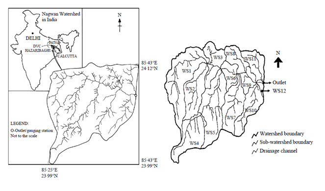
Fig. 32.1. Location and Sub-watersheds Delineated Nagwan watershed in India. (Source: Kaur et al., 2004)

The proposed SDSS comprises of a hydrological model- Soil and Water Assessment Tool (SWAT).  The SWAT Arc-View system consists of three key components:

1. Generating sub-basin topographic parameters and model input parameters

2. Editing input data set and executing simulations

3. Viewing graphical and tabular results.

The delineation of the watershed and the development of the watershed and sub-watershed database were the first set of fundamental steps performed by the proposed SDSS. The watershed and its sub-watershed boundaries were delineated from the DEM of the test area (Kaur and Dutta, 2002) by setting a threshold value of 300 ha or 834 cells for starting the stream delineation. This led to the delineation of 12 sub-watersheds within the watershed (Fig. 32.1). This was followed by determination of all the geometric parameters of sub-basins and stream reach by means of the raster-grid functions of the GIS. These were stored as attributes of derived vector themes. Next, the land use and soil grids and the related data files were loaded and clipped in the watershed area followed by their re-classification and re-sampling at the DEM cell size. In order to capture the heterogeneity in soil and land-use of the watershed, each sub-watershed within it was further divided into one or more Hydrologic Response Units (HRU), representing a unique combination of the land use and soil types. For example, sub-watershed 1 had 3 HRUs with upland paddy on silty loam soil, upland paddy on loamy sand soil, and long-duration paddy on clay loam soil, while sub-watershed 3 had just 1 HRU with upland paddy on silty loam soil, and sub-watershed 11 had 4 HRUs with corn on sandy loam soil, poor canopy forest on wasteland, upland paddy on loamy soil, and upland paddy on silty loam soil. This resulted in a total of 44 HRUs for the whole test watershed. Precipitation, temperature, and weather-generator data were defined by loading the station location and data files. All the SDSS-required input files were generated sequentially through the interface, and the SDSS was run for the calibration and the validation periods, after setting the initial soil moisture storage and base-flow factor values as 1 and using the Pristley–Taylor method for evapotranspiration estimations. Formulation of an LP model for the optimized land-use plan, a Linear Programming (LP) technique, which has been used since the late 1950s in a wide variety of planning situations (Dantzig, 1963), was used to design a model to propose an optimum land-use plan for the watershed.

Defining Decision Variables

Any LP analysis starts by defining ‘decision variables’, which are the different alternatives stated by the problem; for example, in a land-use planning situation, the decision variables may be the different land-use types (LUTs) to be allocated. Strictly speaking, LP is not a spatial technique, because it does not take into account the spatial distribution of the decision variables. However, it can be tailored to deal with spatial problems, if previous regionalization is performed by means of any GIS tool in a SDSS. In the present investigation, in order to capture the soil, land-use, topography, and climate heterogeneity (the four important variables controlling soil and water loss) in a watershed, the delineated watershed was divided into 15 sub-watersheds and 44 HRUs using the Arc-View GIS and the Arc-View Spatial Analyst packages. In the proposed LP algorithm, these individual HRUs were treated as decision variables, representing specific land use types under a specific soil type in a particular sub-watershed in the test watershed. By doing so, it was possible not only to take into account the spatially distributed character of constraints, to obtain more practical and realistic plans for reduced total soil and water losses from the watershed, but also to spatially distribute the LP-optimized resource plan (i.e. different land-use types) for better planning and decision-making.

Establishing objectives is in fact the most important step of any LP analysis, as it is the definition of the objectives that guides the decisions to be taken for solving the problem. Often, these objectives are mutually contradictory, so they can be conceived as either objectives or constraints. In the present exercise, the main objective of planning new land uses was to reduce the total soil loss from the watershed. Thus, the objective here, in a way, was to maximize the most soil loss reducing land-use type(s). This objective function (Z); i.e. minimization of total soil loss (in tonnes) from the watershed was hence expressed as:

 

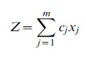
where: the x_j values are the decision variables, each representing the total (optimized) area (ha) under a given LUT in a j^th (with j=1, 2,… m; m=44) HRU within the watershed, and the c_j values refer to the (known) soil loss rates (t/ha) from each of these HRUs under a given LUT (and soil and topography). These c_j values can be either the actual plot-experiment-based soil-loss values under each LUT or the values simulated through a well-tested and validated hydrologic model. Under real-world conditions, it is not practical to obtain actual soil-loss values, under varying soil, climate, and topographic conditions, for each LUT through field/plot experiments. Hence, in the present exercise (case study), these c_j values represented the proposed SDSS-estimated, 9-year (validation period) averaged (Kharif season), soil-loss values for each HRU within the watershed under existing resource-management conditions.

Identifying Key Constraints

The above objectives are constrained by economic, resources, and environmental limitations as well as by a set of secondary objectives. For this exercise, three sets of constraints were considered. These constraints were ecological (soil loss constraints), technical (paddy-yield, corn-yield, labour, affinity for forest and total area constraints), and financial (benefit from paddy and corn cultivation). Since the proposed land-use (LU) planning model was designed only for the Kharif season (i.e. the season with maximum soil and water loss from the region), the major LUTs considered in the proposed LU-optimization problem for the area were forests, paddy, and corn. These constraints, for the proposed land-use planning LP model, were mathematically expressed as detailed in the following subsections.

Sub-Watershed Area Constraints

In general, soil losses are minimal from areas under forest covers. Hence, designing a single area constraint for the whole watershed, with 44 decision variables, each representing an HRU with either (long-duration Kharif or upland) paddy, upland corn or forest (open or closed) would have led to a vast allocation of forested area in the test watershed, thereby leading to a infeasible land-use plan for the area. To take care of this problem, each sub-watershed was considered to be a compact and self-sufficient unit as far as the selection of LUTs was concerned. By doing so, land-use allocations within a watershed were restricted to only the LUTs found within each sub-watershed. This was expressed in the form of the following 15 sub-watershed area constraints in the proposed land-use LP model:

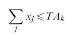
where: TA_k=total (known) area of the k^th (with k=1, 2,…. 15) sub-watershed (in ha), as obtained from the SWAT-Arc View interface of the proposed SDSS; and x_j = (optimized) area under a given LUT in (one or more) j^th HRU(s) in a k^th sub-watershed.

Sub-Watershed Soil-loss Constraints

Soil loss rate (s_j) is a function of land topography, physiography, climate, and hydrology. Hence, it was considered to be an important (integrated) index constraining suitability of a land under a particular land-use type. The total soil loss from a watershed is a function of soil loss from each HRU in a sub-watershed. Thus, to minimize the total soil loss from the watershed, following 15 sub-watershed soil loss constraints were designed so as to constrain the total soil loss per HRU (or a decision variable or a LUT), within a particular sub-watershed, to either less than or equal to the total (current) soil loss from that sub-watershed. These 15 soil-loss constraints were expressed as:

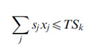
where: TS_k=total (known) current soil loss (in tonnes, during the Kharif season) from the k^th (with k=1, 2, … 15) sub-watersheds, as obtained through the hydrologic component of the proposed SDSS; x_j=(optimized) area under a given LUT in a j^th HRU (ha) in the k^th sub-watershed; and s_j=the current soil loss rate (t/ha) under a given LUT in a j^th HRU in the k^th sub-watershed.

Yield Constraint for Paddy

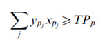
where: x_pj=(optimized) area (ha) under a paddy in a (presently paddy producing) j^th HRU in the test-watershed, and y_pj=current paddy yield (t/ha) in a (presently paddy producing) j^th HRU in a test watershed under existing resource-management practices. These y_pj values can be either the actual plot-experiment-based paddy yield values under each soil type and climatic and management conditions or the values simulated through a well-tested and validated crop model. In real-world conditions, it is not practical to obtain actual paddy-yield values, under varying soil, climate, and topographic conditions through actual field/plot experiments. Hence, in the present exercise, these y_pj values represented the proposed SDSS estimated, 9-year (validation period) averaged (Kharif season), paddy-yield values for each HRU in the test watershed under the existing resource-management practices. These (simulated) paddy-yield values estimated through the proposed SDSS for each HRU within the test area were observed to be ranging between 0.74 and 0.94, with an average of about 0.901 t/ha for the whole test area. Thus, in the above expression, TP_p=total (current) paddy productivity (in tonnes) in the watershed was equated to 0.901 t/ha x 5898 ha (i.e. total current area under paddy cultivation) = 5299.8 tonnes.

Yield Constraint for Corn

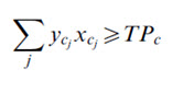
where: x_cj=(optimized) area (ha) under corn in a (presently corn producing) j^th HRU in the test watershed, and y_cj=current corn yield (t/ha) in a (presently corn producing) j^th HRU in the watershed under existing resource-management practices. Like paddy yields, these were also estimated through the proposed SDSS for each HRU within the watershed. It has been observed that these ranged from 0.189 to 1.904, with an average of about 0.907 t/ha for the whole test area. Thus, in the above expression, TP_c = total (current) corn productivity (in tonnes) in the watershed was equated to 0.907 t/ha x 725.7 ha (i.e. total current area under corn cultivation) = 658.21 tonnes.

Benefit Constraint for Paddy

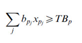
where: x_pj=(optimized) area (ha) under paddy cultivation in a (presently paddy producing) jth HRU in the watershed, and b_pj=current benefit (of Rs 1010.28 per ha, obtained as per the collected economics of the area through PRA exercise) with paddy cultivation in a (presently paddy producing) jth HRU in the watershed. Based on this, TB_p=total (current) benefit with paddy cultivation in the watershed was equated to 1010.28 (Rs per ha) x 5898 ha = Rs 5958631.4, as shown in Table 32.1.

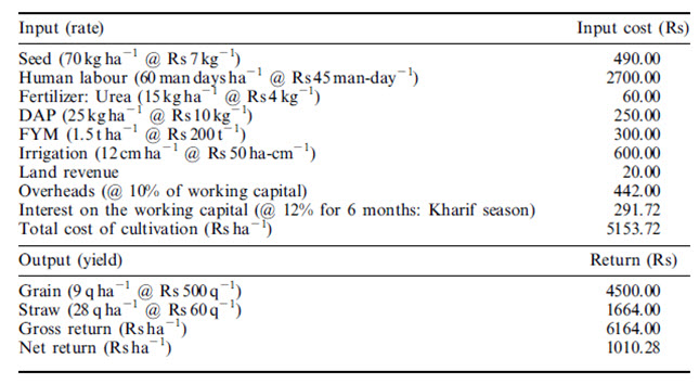
Table 32.1. Cost Benefit Analysis of Paddy Cultivation in the Watershed

(Source: Kaur et al., 2004)

Benefit Constraint for Corn

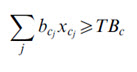
where: x_cj = (optimized) area (ha) under corn (or corn) cultivation in a (presently corn producing) j^th HRU in the watershed, and b_cj=current benefit (of Rs 3639.34 per ha, obtained as per the collected economics of the area through PRA exercise) with corn cultivation in a (presently corn producing) j^th HRU in the watershed. Based on this, TBm=total (current) benefit with corn cultivation in the watershed was equated to 3639.34 (Rs per ha) x 725.7 ha = Rs 2,641,069, as shown in Table 32.2.

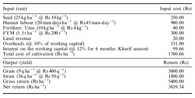
Table 32.2. Cost Benefit Analysis of Corn (Maize) Cultivation in Nagwan Watershed(Source: Kaur et al., 2004)

Labour Constraint

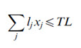
where: x_j=(optimized) area under paddy or corn cultivation in a j^th HRU (ha) in the test watershed; l_j=labour required for paddy (=60 man-days/ha) or corn (=20 man-days/ha) cultivation in a j^th HRU with paddy or corn cultivation, respectively, in the watershed; and TL=total labour (man-days) available in the watershed (i.e. total agricultural labour-number of days in the 5-month growing season=10034 x 5 x 30 = 1505100), as per the collected economics of the area through PRA exercise.

Affinity Constraint for Forest

This was designed to maintain at least the current level of forested area (i.e. 30% of the total area) in the watershed:

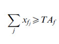
where: TA_f = current total area under forest cover in the watershed (=2850 ha), and  xf_j~(optimized) area (ha) under forest cover in a (presently forested) j^th HRU in the watershed.

Total Watershed Area Constraint

This was designed to ensure that the sum of areas allocated, by the proposed LP model, to all HRUs within watershed is never more than the total watershed area.

where: TA~actual total area (ha) of the watershed (~9576 ha), and x_j~(optimized) Area (ha) under each land-use type in a j^th HRU in the watershed.

Implementation of the LP Model

After obtaining the necessary coefficients as detailed in the previous section, the objective function and the constraints for the proposed LP model were designed and implemented on a standard MS-DOS personal computer and public-domain software, QSB (Quantitative Systems for Business V 2.0; Chang and Sullivan 1986). The input matrix for the proposed land-use LP model was solved in 32 iterations.

Results and Discussion

SDSS proposed sediment yields under the existing land-use plan, the calibrated available soil water capacity and curve number values. The proposed SDSS yielded a moderately good correlation coefficient and model efficiency coefficient values of 0.54 and 20.67, respectively for the observed versus predicted total sediment yields for the calibration years. The observed data for the validation period indicated an annual average total sediment yield of 25.35 t/ha from the Nagwan watershed during the Kharif seasons. In comparison with this, the proposed SDSS predicted an annual average total sediment yield of 21.28 t/ha, with a correlation coefficient of 0.65, model efficiency of 0.70, relative error of 217.97%, and root mean square prediction error of 9.63 t/ha for the same validation period. The above results clearly showed that, even under Indian conditions, with data sets of poor spatial resolutions, the proposed SDSS could simulate the annual dynamics of the total sediment yield at the watershed outlet reasonably well. Hence, it was assumed that the proposed SDSS was capable of mimicking even HRU and sub-watershed-scaled sediment yields realistically.

LP Model Proposed Sediment Yields Under the Optimized Land-use Plan

On comparing the total sediment yield values under the LP-optimized alternate land-use plan (18.11 t/ha) with those under existing land use (21.28 t/ha), it can be seen that the LP-optimized land-use plan could lower the total sediment yield from the watershed by about 14.89%. SDSS proposed sediment yields under the LP model proposed optimized land-use plan. Incorporation of the LP model proposed land-use plan in the proposed SDSS resulted in an average annual total (Kharif season) sediment yield of 18.17 t/ha, as compared with the 21.28 t/ha under the existing land-use plan, for the 9-year validation period. It could be clearly seen that even the proposed SDSS predicted an annual average reduction of 14.61% in the total watershed sediment yield under the LP-optimized land-use plan. This decrease could also be seen at the sub-basin level from the annual average spatial distribution map of the test watershed. Besides this, the proposed land-use plan resulted in an increase in the paddy (0.926 t/ha) and the corn (1.523 t/ha) crop yields in the watershed by 2.80 and 68.14% over the present paddy (0.901 t/ha) and corn (0.907 t/ha) crop yields, respectively.

Conclusions

The present investigation could thus quite realistically demonstrate the potential of the proposed SDSS for assessing the impact of on-going resource management practices on the sediment yields from the Nagwan watershed simply meaning the value of land use land cover optimization benefit. Besides this, it also demonstrated the immense application potential of such spatial decision support systems in designing an LP-optimized regional soil conserving-land-use plan and assessing its impact on the total sediment yield from the watershed.

32.2 Case Study on Optimal Land Use Outside India

Study Area

The Brimvand watershed is located in upstream of agricultural canal of Brimvand dam and 4 km from north of Sarpole Zahab City in Kermanshah Province, Iran. It comprises 9572 ha area distributed within 15 sub-watersheds as shown in Figure 32.2.

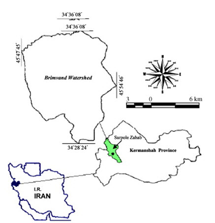
Fig. 32.2. Study Area Location. (Source: Sadeghi et al., 2009)

Data Acquisition and Problem Formulation

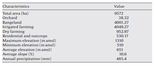
The problem was structured in the study area to maximize economic return and minimize soil loss. The information and data required for defining constants and coefficients of objective functions and constraints, viz. land availability, water availability/supply, soil characteristics, slope steepness and aspect, present land use, soil erosion and sediment yield, socio-economical conditions were extracted from the available comprehensive studies (Kermanshah Watershed Management Office, 2000) conducted for the area. The geographical characteristics of the study area are given in Table 32.3. 

Table 32.3. The Important Geographical Characteristics of the Brimvand Watershed in Iran (Source: Sadeghi et al., 2009)

 

In addition to the above-mentioned information, some other field studies and land surveys were also conducted for checking, and further details and information. The general benefit maximization problem was formulated as below:

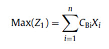
Where, Z₁ is the total annual income in million Iranian Rails (mIR), C_Bi is annual income for each land use (mIR/ha), Xi is the area of each land use in ha and n stands for numbers of land uses. If the annual gross benefit, production cost and soil erosion destruction cost per hectare of different land uses is given by A_i1, A_i2 and A_i3, the above equation can be rewritten as below.

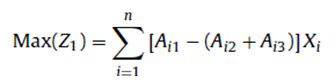
where, A_i1 is the gross profit for every land use, A_i2 is the production costs spent for each land use and A_i3 represents the costs wasted on soil caused by erosion in every land use.

The second objective was to minimize soil erosion as represented in the following equation:

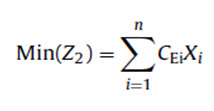
where, Z₂ = total soil erosion (t year^-1), C_Ei = annual soil erosion for every land use (t ha^-1 year^-1), X_i = the area of each land use (ha), i = the land use number and n = the total number of land uses. Within the watershed, following were the considered land capability constraints:

X1 ≤ B1                                                                                                     

X3 ≤ B2                                                                                                     

X4 ≤ B3                                                                                                     

X1 + X3 ≤ B4                                                             

The land availability constraints were considered as below:

X1 + X2 + X3 + X4 ≤ B5                                                                          

The considered social and legislation constraints were like below:

X1 ≥ B6                                                                                                     

X2 ≥ B7                                                                                                     

Non-negativity constraints to solve the LP model were as below:

X1, X2, X3 and X4 ≥0                                                                              

Where, B1 to B4 are the maximum allowable area to orchard (X1), irrigated farming (X3), dry farming (X4), and summation of orchard and irrigated farming. B5 denotes the maximum arable land resources. B6 and B7 represent the minimum area of orchard and rangeland (X2) in ha respectively. Since there are sufficient and accessible water supply systems in Brimvand watershed, no constraint was defined for water availability. There are 10 springs with discharges from 2 to 453 l/s (16.9 Mm³/year) and 128 wells with the total discharge capacity of 11.2 m³/year in the study watershed. The main irrigation canal of Brimvand Dam with the average discharge of 5 m³/s also passes along the entire watershed. The above objective functions and constraints were quantified in coordination with site-specific information, which directly or indirectly obtained for the study area. Since the economic losses resulting from soil erosion have also to be considered in the first objective function, the soil erosion estimation in different land uses was conducted on the first onset. The estimation of soil erosion was made using Pacific South-West Interagency Committee method for 15 hydrologic units after applying the concept of sediment delivery ratio. The model consisted of nine factors, viz. surface geology, soil erodibility, climate, runoff, topography, vegetation cover, land use, upland erosion and gully erosion which were totally determined for the entire sub-watersheds. The erosion estimates were then incorporated to the land uses existed either thoroughly or partially in each hydrologic unit (sub-watershed) and the soil erosion rate associated with each land use was ultimately found out. The possible land use modification was then incorporated in order to minimize soil erosion rate based on land capability criteria and cultural, social and legal constraints.

The annual gross benefit, production cost and soil erosion destruction cost per each hectare of different land uses were estimated according to Kermanshah Watershed Management Office  studies and interviews made with the inhabitants. Based on the collected data and information, grape is the main orchard product planted in terraced lands. There is no interest among the watershed inhabitants to invest on gardening for long term period return. Meanwhile, the farmers are not convinced to have commercial gardening through which they can be benefited. The low level economic conditions of the watershed inhabitants make them to scare large investments with high risk. The individual contracts between almost two thirds of the farmers and the landowners to guarantee the low but reliable income are one of the evident of such unreliable benefit to the farmers. The irrigated areas are mainly used for wheat, corn, melon, alfalfa, cotton, and bean plantation. Wheat, barley and peas are cultivated in dry farming areas as well under low tillage precaution. They usually prefer dry farming land use, since according to them, it needs low attention and tillage activities through which they also ascertain their ownership. The rangeland areas are also mostly being utilized for sheep and goat grazing purposes and the rates of benefits were then calculated based on the forage productions and the total digestible nutrients (TDN), which feeds a particular number of animal units. The dry forage production amounts of less than 50, 50–120 and more than 120 kg/ha were considered for rangeland classification in three categories of light, moderate and heavy grazing. Erosion destruction cost was estimated by calculating the area lost to erosion in each land use considering rooting depth and soil bulk density. The coefficients of maximization objective function were ultimately calculated using net benefit obtained through subtracting total cost from gross benefit. The right hand side values of the constraint equations were then determined based on land capability standards defined according to slope steepness, soil depth and water availability as well as cultural and legal constraints with the help of geographic information system. The benefit maximization and soil erosion minimization in the Brimvand watershed were solved with the help of ADBASE model which is capable to solve multi-objective problems using the simplex method. In order to obtain the most effective constraint as well as land use on changing objective functions, which facilitates decision makers/managers to address various alternatives (Chang et al., 1995), the sensitivity analysis was also performed through subjecting the objective functions to a particular change of input resources within the permissible range of variation. The permissible ranges were approximately assigned with respect to the potential of change of the variables under consideration. The percentiles of changes were then depicted against each other’s and the most sensitive land use was ultimately distinguished in both objective functions.

Application of the Model to Brimvand Watershed

As already explained, only two broad planning objectives of economic development and soil erosion reduction were considered to be optimized in the Brimvand watershed. The soil erosion rates were estimated to be 7.39, 8.14, 7.39 and 21.11 t/ha/year for orchard, rangeland, irrigated farming and dry farming land uses, respectively. Since, the rooting depth and soil bulk density in orchard, rangeland, irrigated farming and dry farming land uses based on field studies and lab experiments were measured to be 1.00±0.2, 0.15±0.05, 0.50±0.1 and 0.15±0.06m, and 1.08±0.04, 1.11±0.06, 1.08±0.07 and 1.09±0.05 t/m³, respectively, the area depleted owing to soil erosion found to be 6.84±1.7, 48.91±7.0, 13.68±3.2 and 129.13±16.6 m²/year per each unit area (ha) of land uses at sequence. The mean net benefit of orchard, rangeland, irrigated farming and dry farming land uses were therefore calculated as 8.50, 0.16, 4.88 and 0.32 mIR/ha, respectively. So that, the objective functions of the benefit maximization and the soil erosion minimization problems in the Brimvand watershed were formulated as follows:

Max (Z₁) = 8.5042X1 + 0.1562X2 + 4.8758X3 + 0.3215X4                    

Min (Z₂) = 7.389X1 + 8.144X2 + 7.389X3 + 21.112X4                 

The above two objective functions were then subjected to the following constraints. Considering no limitation for water availability for all land uses, the maximum allocation of  area of 518.81 with slope below 12% and soil depth beyond 0.65 m was contemplated for orchard as,

X1 ≤ 518.81                                                      

Almost 59% of the area lies between altitude ranges of 500–600 m above mean sea level (msl). Most of the watershed appears as hilly, plateaus and alluvial fan land types. The slope of some 38% of the area is below 2%. The maximum area of 4044.64 ha could therefore be designated for irrigated agriculture with slope below 5% and very deep soil (>100 cm). Thus the constraint was formulated as below:

X3 ≤ 4044.64                                                                    

The upper slope limit of 12% based on the existing standards and government regulation was applied for determining the maximum allocation of land for dry farming agriculture as given below:

X4 ≤ 1464.34                                                                   

Based on the similarities between recommended standards for irrigated and orchard land uses and easiness of having access to water resources, the following constraint was also formulated for the study area.

X1 + X3 ≤ 4563.37                                               

It was not possible to change the utility of inhabitant, roads and outcrops areas and these areas had to be therefore subtracted from the entire watershed area and the rest area was used for optimization. In the other words, the total land available for development in the watershed was 9041.83 ha. That was

X1 + X2 + X3 + X4 ≤ 9041.83                         

According to the current cultural tendency of the people in this region toward household gardening mainly for self-sufficiency and amusement, the area under orchards could be limited at least at the level of existing area of 38.32 ha.

X1 ≥ 38.32                                                                        

Government regulation, Iran Forest and Rangeland Nationalization Act of 56 required that the rangeland area should be legitimately no less than 4001.27 ha in this watershed for the purpose of natural resources conservation. Therefore,

X2 ≥ 4001.27                                                                     

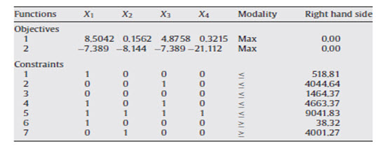
The corresponding simplex method table was therefore extracted according to the formulated problem for the study watershed as given in Table 32.4.

Table 32.4. Simplex Table for Land Use Optimization in Brimvand Watershed, Iran (Source: Sadeghi et al., 2009)

Optimization Results and Analysis

From Tables 32.3 and 32.4, it can be seen that there is no serious change in irrigated farming and rangeland areas, whereas the orchard area with a very small quantity of land occupancy has been increased by 13.5 times and the dry farming area has been declined by 50%. All these possible changes can be made within the areas qualified for each land use as depicted in Fig. 32.1. It is environmentally as well as economically preferred that some uses, mostly dry farming land use, to be changed to orchards, since the steep slope areas with high erosion rate and less production is traditionally converted to level terraces by the farmers when they develop orchards. Further, prior to change, the land needs to be precisely surveyed to avoid any hazardous unexpected problem. The linear optimization problem was successfully solved using the multipurpose ADBASE software program. The results also showed the successful linkage between economic aspects and environmental outcomes at a watershed scale. Because of changes considered in land use areas through optimization, the annual benefit enhanced from 21,001 to 24,911 mIR (i.e. 18.62% growth), whereas the annual soil erosion would decrease from 82,910 to 76,380 t (i.e. about 7.87% reduction). Such type of land use allocation not only satisfied all governing constraints exist in the study watershed but also ascertained socio-economic improvement, legitimate fulfillment and environmental sustainability.

Sensitivity Analysis

The sensitivity analysis was also performed for the benefit maximization as well as soil erosion minimization objective functions and the corresponding results have been depicted in Figs. 32.3 and 32.4, respectively. Scrutinizing the results of sensitivity analyses (Figs. 32.3 and 32.4) verify that the changes in objective functions in both cases are linear and they are mostly controlled by reduction in rather than increasing the resources. It can also be verified here that the change of some specific allocations would create much more impact on the final optimal solutions generated by the optimization programming in connection with variations of parameter values versus the relative changes of decision variables. It could also be implied from Fig. 32.3 that reduction in benefit has the highest sensitivity to the reduction of orchard and irrigated farming areas, whereas benefit increment is only sensitive to increase in orchard area. It is seen in Fig. 32.4 that the reduction of irrigated farming and orchard areas increased soil erosion drastically. On the other hand, reduction in rangeland area leads to increase soil erosion. In over all, the changes in benefit and soil erosion in Brimvand watershed is mainly controlled by variation in orchard and irrigated land uses.

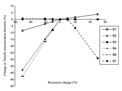
Fig. 32.3. Sensitivity Analysis of Benefit Maximization Function in Brimvand Watershed, Iran (B1, B2, B3, B4, B6 and B7 are Maximum Allowable Area to Orchard, Irrigated Farming, Dry Farming, Summation of Orchard and Irrigated Farming, Minimum Area of Orchard and Rangeland, Respectively). (Source: Sadeghi et al., 2009)

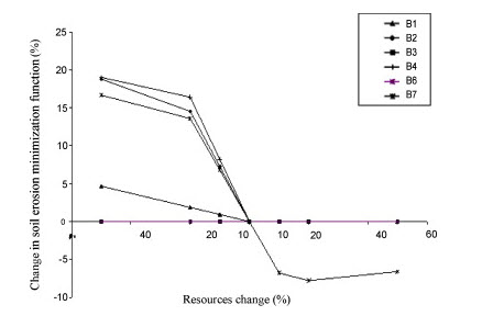
Fig. 32.4. Sensitivity Analysis of Soil Erosion Minimization Function in Brimvand Watershed, Iran (B1, B2, B3, B4, B6 and B7 are Maximum Allowable Area to Orchard, Irrigated Farming, Dry Farming, Summation of Orchard and Irrigated Farming, Minimum Area of Orchard and Rangeland, Respectively). (Source: Sadeghi et al., 2009)

Conclusion

A benefit and soil erosion problem was formulated and solved to minimize soil erosion and maximize benefits using optimization of allocation of  land resources to orchard, range, irrigated and dry farming land uses within the Birmvand watershed in Kermanshah province, Iran. The ADBASE optimization software program was successfully applied and led to determine appropriate areas allotted to different land uses. The results obtained during the study approved the applicability of optimization model in solving problems, which sometimes conflicting each other. It can also be concluded that contrary to single objective classical land use planning models, the multi-objective linear programming can be used to tractably search for optimum land use scenarios with respect to different governing constraints existing within a watershed. On the study watershed there appears a significant reduction in soil erosion and augmentation in profit from allocating the optimal land uses.

Keywords: Optimal Land Use, Watershed Processes Simulation, Case Studies, India.

References

• Sadeghi, S.H.R., Kh. Jalili & D. Nikkami, (2009). Land Use Optimization in Watershed Scale. Land Use Policy, 26: 186-193.

• Kaur, R., Srivastava, R., Betne, R., Mishra, K., & Dutta, D. (2004). Integration of Linear Programming and a Watershed-Scale Hydrologic Model for Proposing an Optimized Land-Use Plan and Assessing its Impact on Soil Conservation-A Case Study of the Nagwan Watershed in the Hazaribagh District of Jharkhand, India. International Journal of Geographical Information Science, 18(1): 73-98.

Suggested Readings

• Verburg, P. H., Schot, P. P., Dijst, M. J., & Veldkamp, A. (2004). Land Use Change Modelling: Current Practice and Research Priorities. GeoJournal, 61(4), 309-324.

• Lillesand, T. M., Kiefer, R. W., & Chipman, J. W. (2004). Remote Sensing and Image Interpretation (No. Ed. 5). John Wiley & Sons Ltd.

• Jensen, J. R. (2009). Remote Sensing of the Environment: An Earth Resource Perspective 2/e. Pearson Education India.