Site pages
Current course
Participants
General
Module 1. Moisture content and its determination.
Module 2. EMC
Module 3. Drying Theory and Mechanism of drying
Module 4. Air pressure within the grain bed, Shred...
Module 6. Study of different types of dryers- perf...
Module 5. Different methods of drying including pu...
Module 7. Study of drying and dehydration of agric...
Module 8. Types and causes of spoilage in storage.
Module 9. Storage of perishable products, function...
Module 10. Calculation of refrigeration load.
Module 11. Conditions for modified atmospheric sto...
Module 12. Storage of grains: destructive agents, ...
Module 13. Storage of cereal grains and their prod...
Module 14. Storage condition for various fruits an...
Module 15. Economics aspect of storage
Lesson 5. Emc Curve And Emc Models
5.1 Sorption Theory
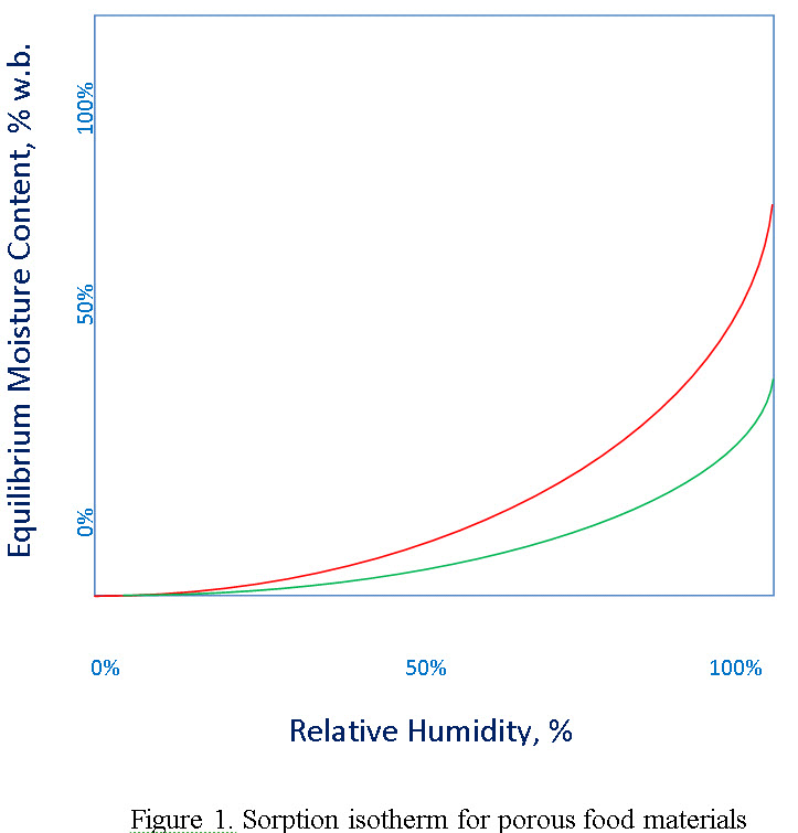
EMC data for dry food which is generally hygroscopic material, describe the material’s moisture content originating from an interaction with the moisture and temperature of the surrounding air. If a dry food is placed in environment with a constant humidity and temperature, it will take up moisture by adsorption until it reaches its equilibrium moisture content (where the net moisture exchange is zero) which is called as adsorption EMC. If, however, a wet food with the same properties is placed in the same environment, it will loose moisture by desorption and reach to equilibrium moisture content which is called as desorption EMC. For each product the relative humidity of environment can be changed and different adsorption and desorption EMC values can be obtained. If these values are plotted on a graph a loop is obtained which is called hysteresis (Figure 1). The hysteresis effect is observed due to shrinkage effect during desorption which changes the water binding properties of the food product. Therefore, during adsorption same path of EMC is not observed.
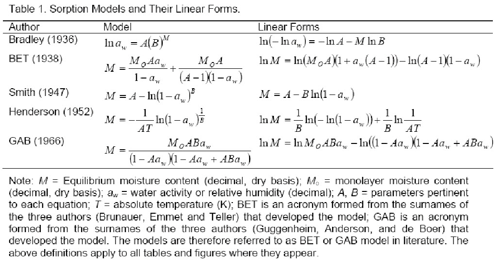
5.2 EMC Models
Equilibrium moisture content (EMC) relationships are required to achieve target moisture contents (MC) during the grain conditioning process. ASAE Standard D245.5 provides EMC models for popcorn grains along with the parameter values for the desorption process. However, the accuracy of these values have been found to be inadequate to tightly control fans and heaters during automatic grain conditioning, which can result in huge losses especially in high value crops such as popcorn.
There are several models available for different foods to predict the EMC.
They are as follows:
-
Kelvin Model
Kelvin in 1871 developed EMC model based on the condensation in capillary. He developed relationship between vapour pressure over liquid in capillary (Pv) and the saturated vapour pressure at the same temperature (Pvs), the relationship is as follows:
\[\ln\left({\frac{{Pv}}{{Pvs}}}\right)=-\frac{{2\sigma V\cos \alpha }}{{rRoTabs}}{\rm{ }}\]
Where Pv is the water vapor pressure of the product, Pvs is the saturated water vapour pressure at the equilibrium temperature of the system, σ is the surface tension of the moisture, V is the volume of the moisture in liquid form, r is the cylindrical capillary radius and α is contact angle between moisture and capillary wall.
2. Langmuir model
3. BET equation
4. Harkins-Jura equation
5.GAB equation