Engineering Properties of Biological Materials and Food Quality 3(2+1)

Lesson 7. Aerodynamic properties of biomaterials

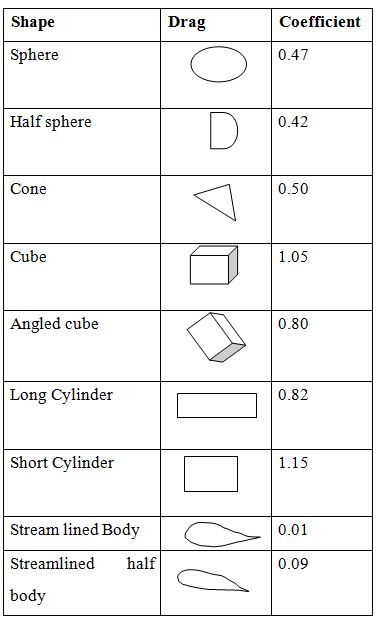
7.1. Drag Coefficient:-

It is used to quantify drag or resistance of an object is a fluid environment such as air or water. It is a dimensionless quantity. Drag coefficient is always associated with surface area:

Figure

 

 

 

 

 

 

 

 

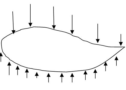
When fluid flow occurs about immersed objects, the action of the forces involved can be illustrated as follows. The pressure of the upper side of the object is less than that of lower side is great than that of & that of lower side is greater than the pressure p in the undisturbed fluid stream. In addition to these force normal to the surface of the object, there are shear stresses, C acting tangential to the surfaces in the direction of flow & resulting from frictional effects.

 The resultant force for may be resolved into components, F_D the drag & F_V the lift force.

\[{F_D} = {f_1}({A_P},{\rho _f},\eta ,E,V)\]   \[{A_P}\]=Projected area of the object

\[{F_L} = {f_2}({A_P},{\rho _f},\eta ,E,V)\]   r_f=Fluid density,  h=Viscosity of fluid                                    

E= modulus of Elasticity

 V= Velocity of the object relative to fluid

Employing dimensional analysis.

\[{F_D} = {C_D}\frac{{{A_p}{\rho _f}{V^2}}}{2}.............................1\]

\[{F_L} = {C_L}\frac{{{A_p}{\rho _f}{V^2}}}{2}.............................2\]

 \[{C_D}\] &\[{C_L}\]   are drag coefficient & lift Coefficient

\[{F_r} = \frac{1}{2}C{A_p}{\rho _f}{V^2}.............................3\]

\[{F_r}\]=resistance drag force Wt. of particles at   thermal velocity

C= overall drag coefficient

 In certain cases it is desirable to resolve the resultant force into components of force into components of frictional drag to tangential force on the body surface & profile drag due to pressure distribution around the body. In laminar or low velocity flow where variation in fluid density is small and viscous action governs the flow, the profile or pressure drag is negligible. In thermal or high velocity flow where fluid compression & not viscous action governs the flow, the frictional drag is negligible.

e.g. Frictional drag:- drag force exerted on one side of a smooth flat plate aligned with flow.

e.g.  Profile drag:- drag force on blunt object.

Frictional Drag: - for Flat laminar boundary layer

\[{C_f} = \frac{{1.328}}{{{{\left( {{N_R}} \right)}^{0.5}}}}............4\]

For flat plate turbulent boundary layer

\[{C_f} = \frac{{0.455}}{{\log {{\left( {{N_R}} \right)}^{2.58}}}}............5\]

\[{N_R}\]=Reynolds number \[{N_R} = \frac{{Vdpf}}{\eta }.....................6\]

d=length or diameter of a sphere (dimension of an object)

η=absolute viscosity,

V= relative velocity

r_f= fluid density

For transition region

\[{C_f} = \frac{{0.455}}{{\log {{\left( {{N_R}} \right)}^{2.58}}}} - \frac{{1700}}{{{N_R}}}............7\]    Drag should be multiplied by 2 for plates of 2 side.

Profile or Pressure Drag:

When a blunt object, known as sphere is placed in a fluid flow, the frictional drag can be neglected because of the small surface area on which frictional effects can work. The exception is the case of flow at very low Reynolds number is less than unit, where stokes low is applicable. Here inertia force may be neglected & those of viscosity alone considered, the flow closes behind a sphere like object & profile drag is composed primarily of frictional drag.

Stoke’s law of drag force

 \[F\Delta  = 3\pi \eta V{d_P}...........8\]     \[{d_P}\]= diameter of sphere, diameter of sphere,

viscosity

Equating (9) equation (1)

\[{F_D} = \frac{{{C_D}{A_P}{\rho _f}{V^2}}}{2} = 3\pi \eta V{d_p}\]

\[3\pi \eta V{d_p} = \frac{{{C_D}{A_P}{\rho _f}{V^2}}}{2}\]  \[{N_R} = \frac{{\rho V{d_p}}}{\eta }\]

\[3\pi \eta {d_p} = \frac{{{C_D}{\pi ^2}}}{{2 \times 4}}d_P^2{\rho _f}V\]  \[{A_P} = \frac{\pi }{4}d_p^2\]

24=C_DN_R  \[24 = {C_D}{\rho _f}\frac{{V{d_P}}}{\eta }\]

\[{C_D} = \frac{{24}}{{{N_R}}}...............9\]

As Reynolds number exceeds unity, the stokes law is no longer applicable because flow opens up behind the blunt object & the drag force is a combination of frictional drag as well as pressure drag in a range up to N_R =1000. N_R above frictional effect may be negligible.

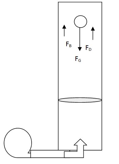
Terminal Velocity:

In free fall, the object will attain a constant terminal velocity V_t at which, where acceleration will be zero.

Net gravitational accelerating net upward equals to the sum of buoyant force and drag force

Gravitational force acting downward= buoyant force exerted by the fluid on the body in upward direction+ drag force (frictional resistance due to motion of the body in the fluid medium)

\[{m_p}g = {m_p}{a_f} + \frac{1}{2}\left( {{A_p}{P_f}V{t^2}} \right)........10\]

\[{m_p}g\left( {\frac{{{\rho _p} - {\rho _f}}}{{{\rho _p}}}} \right) = \frac{1}{2}\left( {{A_p}{\rho _f}V{t^2}} \right)........10\]    g= acceleration due to gravity

\[{V_t} = \left[ {\frac{{2W({\rho _p} - {\rho _f})}}{{{\rho _f}{\rho _p}{A_P}C}}} \right]\]  g= acceleration due to gravity

\[{V_t} = \left[ {\frac{{2W({\rho _p} - {\rho _f})}}{{{\rho _f}{\rho _p}{A_P}C}}} \right]\]   \[{m_p}\]= mass of particles, W=wt. of particles

\[e = \left[ {\frac{{2W({\rho _p} - {\rho _f})}}{{{\rho _f}{\rho _p}{A_P}C}}} \right]................11\]   \[{P_p}\]=mass density of particles, \[{P_f}\] =  mass density of fluids

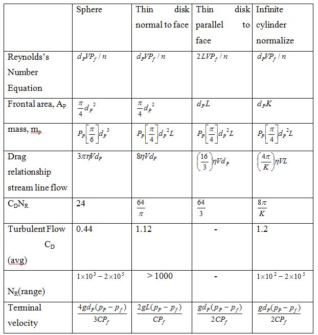
For spherical Bodies

\[{A_p} = \frac{\pi }{4}d_P^2 = W = \left( {\frac{\pi }{6}} \right){P_p}gd_P^3\]

\[{V_t} = {\left[ {4g{d_P}({p_P} - {p_f})/3{p_f}} \right]^{1/2}}..............12\]

For laminar flow, the value of C in calculated from for Reynolds number L1.0, substituting C   in   NR.

\[{V_t} = g{d_P}^2({p_P} - {p_f})/18\eta ..............13\]

For turbulent flow 10³< N_R<2×10⁵ c=0.44

\[{V_t} = 1.74{\left[ {g{d_P}({p_P} - {p_f})/{p_f}} \right]^{1/2}}..............14\]

Finally for intermediate region 2< N_R<10³

\[C = \frac{{18.5}}{{({N_R})0.5}}............15\]

\[{V_t} = \frac{{0.153{g^{0.714}}{d_{}}^{0.142}{{({p_P} - {p_f})}^{0.714}}}}{{{p_f}^{0.286}{\eta ^{0.428}}}}..............16\]

Measurement of terminal velocity:

Most scientists and researchers employ air column to find out the terminal velocity of grains. The set up usually consists of a vertical air column, which is blown from the bottom and passes through the screen. The screen uniformly distributes the air velocity. The air column is also attached with velocity measuring device. The blower maintains variable speed. When grains are allowed to drop into the column, initially they attains acceleration, once the velocity is adjusted they fall to the bottom with a constant velocity. This constant velocity is termed as terminal velocity

Factors affecting aerodynamic properties of biomaterials:

• Frontal area

• Particles size orientation(In turbulent region particles assumes position of maximum resistance)

   

  

L= thickness of disk, length of rod or cylinder length of flat ᶲ late along director of flow

K=2002/n N_R

Grains	Terminal velocity,  m/s
Wheat	9-11.5
Barley	8.5-10.5
Small oats	19.3
Corn	34.9
Soybean	44.3
Rye	8-5-10.0
Oats	8.0-9.0
Grains		Bulk Density		Particle density
Wheat		850		1480-1410
Paddy		575		1411-1342
Parboiled rice		522-566		1405-1346
Rice		507-565		946-991
Bean		750
oat grain				1380.0

 

o   In the handling and processing of agricultural products, air is often used as a carrier for transport or for separating the desirable products from unwanted materials, therefore the aerodynamic properties, such as terminal velocity and drag coefficient, are needed for air conveying and pneumatic separation of materials. As the air velocity, greater than terminal velocity, lifts the particles to allow greater fall of a particle, the air velocity could be adjusted to a point just below the terminal velocity. The fluidization velocity for granular material and settling velocity are also calculated for the body immersed in viscous fluid.

Application to Agricultural products

o   Separation of foreign materials from seeds, grains potato, blue berry
o   Conveying and handling of grains, chopped forage small & large fruits
o   Hydraulic handling of apples, cherries, mango& potatoes etc.

Working principle of Aspirator:- Under steady state condition, where terminal velocity has been achieved, if the particles density is greater than fluid density, the particles motion will be downward. If particles density is smaller than the fluid density, the particle will be rise.