Site pages
Current course
Participants
General
MODULE 1. FLUIDS MECHANICS
MODULE 2. PROPERTIES OF FLUIDS
MODULE 3. PRESSURE AND ITS MEASUREMENT
MODULE 4. PASCAL’S LAW
MODULE 5. PRESSURE FORCES ON PLANE AND CURVED SUR...
MODULE 6.
MODULE 7. BUOYANCY, METACENTRE AND METACENTRIC HEI...
MODULE 8. KINEMATICS OF FLUID FLOW
MODULE 9: CIRCULATION AND VORTICITY
MODULE 10.
MODULE 11.
MODULE 12, 13. FLUID DYNAMICS
MODULE 14.
MODULE 15. LAMINAR AND TURBULENT FLOW IN PIPES
MODULE 16. GENERAL EQUATION FOR HEAD LOSS-DARCY EQ...
MODULE 17.
MODULE 18. MAJOR AND MINOR HYDRAULIC LOSSES THROUG...
MODULE 19.
MODULE 20.
MODULE 21. DIMENSIONAL ANALYSIS AND SIMILITUDE
MODULE 22. INTRODUCTION TO FLUID MACHINERY
LESSON 31. DIMENSIONAL HOMOGENEITY
Dimensional Homogeneity
-
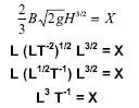
Any equation is only true if both sides have the same dimensions.
-
It must be dimensionally homogenous.
What are the dimensions of X?
-
The powers of the individual dimensions must be equal on both sides.
(for L they are both 3, for T both -1).
-
Dimensional homogeneity can be useful for:
1. Checking units of equations;
2. Converting between two sets of units;
3. Defining dimensionless relationships
- What exactly do we get from Dimensional Analysis?
A single equation, which relates all the physical factors of a problem to each other.
An example:
Problem: What is the force, F, on a propeller?
What might influence the force?
It would be reasonable to assume that the force, F, depends on the following physical properties?
Diameter, d
Forward velocity of the propeller (velocity of the plane), u
Fluid density, ρ
Revolutions per second, N
Fluid viscosity, µ
From this list we can write this equation:
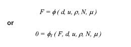
![]()
Dimensional Analysis produces:
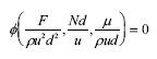
These groups are dimensionless.
Ø will be determined by experiment.
These dimensionless groups help to decide what experimental measurements to take.
These groups are dimensionless.
Ø will be determined by experiment.
These dimensionless groups help to decide what experimental measurements to take.
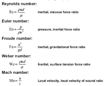
Several groups will appear again and again.
These often have names.
They can be related to physical forces.
Other common non-dimensional numbers or ( π groups):
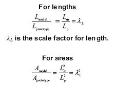
Similarity
Similarity is concerned with how to transfer measurements from models to the full scale.
Three types of similarity which exist between a model and prototype:
Geometric similarity:
The ratio of all corresponding dimensions
in the model and prototype are equal.
All corresponding angles are the same.
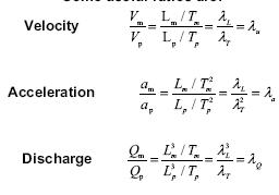
Kinematic similarity :
The similarity of time as well as geometry.
It exists if:
i. the paths of particles are geometrically similar
ii. the ratios of the velocities of are similar
Some useful ratios are:
A consequence is that streamline patterns are the same.
Dynamic similarity
If geometrically and kinematically similar and the ratios of all forces are the same.
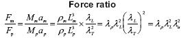
This occurs when the controlling π group is the same for model and prototype.
The controlling π group is usually Re. So Re is the same for model and prototype:
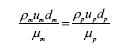
It is possible another group is dominant.
In open channel i.e. river Froude number is often taken as dominant.
Modelling and Scaling Laws
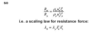
Measurements taken from a model needs a scaling law applied to predict the values in the prototype
An example:
For resistance R, of a body moving through a fluid.
R, is dependent on the following:
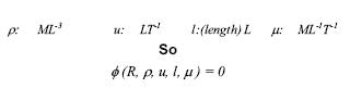
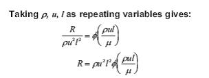
This applies whatever the size of the body i.e. it is applicable to prototype and a geometrically similar model.
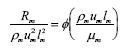
For the model
and for the prototype
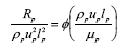
Dividing these two equations gives
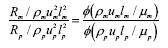
W can go no further without some assumptions.
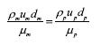
Assuming dynamic similarity, so Reynolds number are the same for both the model and prototype:
Last modified: Tuesday, 8 October 2013, 8:58 AM