Electrical Circuits 3(2+1)

LESSON 9. Network theorems Thevenin’s and Norton’s

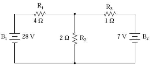
Fig. 9.1

Let’s suppose that we decide to designate R2 as the “load” resistor in this circuit. We already have four methods of analysis at our disposal (Branch Current, Mesh Current, Millman’s Theorem, and Superposition Theorem) to use in determining voltage across R2 and current through R2, but each of these methods are time-consuming. Imagine repeating any of these methods over and over again to find what would happen if the load resistance changed (changing load resistance is very common in power systems, as multiple loads get switched on and off as needed. the total resistance of their parallel connections changing depending on how many are connected at a time). This could potentially involve a lot of work! Thevenin’s Theorem makes this easy by temporarily removing the load resistance from the original circuit and reducing what’s left to an equivalent circuit composed of a single voltage source and series resistance. The load resistance can then be re-connected to this “Thevenin equivalent circuit” and calculations carried out as if the whole network were nothing but a simple series circuit:

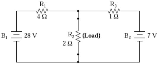
Fig. 9.2

After Thevenin conversion

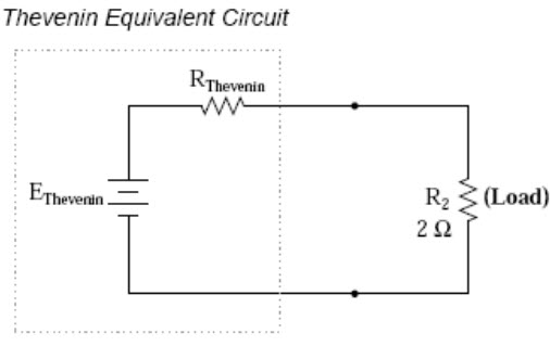
Fig. 9.3

The “Thevenin Equivalent Circuit” is the electrical equivalent of B1, R1, R3, and B2 as seen from the two points where our load resistor (R2) connects. The Thevenin equivalent circuit, if correctly derived, will behave exactly the same as the original circuit formed by B1, R1, R3, and B2. In other words, the load resistor (R2) voltage and current should be exactly the same for the same value of load resistance in the two circuits. The load resistor R2 cannot “tell the difference” between the original network of B1, R1, R3, and B2, and the Thevenin equivalent circuit of E_Thevenin, and R_Thevenin, provided that the values for E_Thevenin and R_Thevenin have been calculated correctly. The advantage in performing the “Thevenin conversion” to the simpler circuit, of course, is that it makes load voltage and load current so much easier to solve than in the original network. Calculating the equivalent Thevenin source voltage and series resistance is actually quite easy. First, the chosen load resistor is removed from the original circuit, replaced with a break (open circuit):

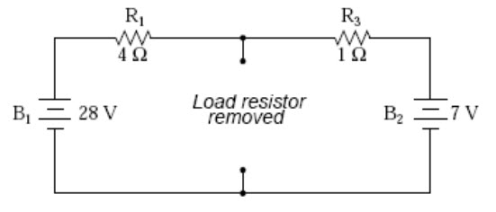
 Fig. 9.4

Next, the voltage between the two points where the load resistor used to be attached is determined. Use whatever analysis methods are at your disposal to do this. In this case, the original circuit with the load resistor removed is nothing more than a simple series circuit with opposing batteries, and so we can determine the voltage across the open load terminals by applying the rules of series circuits, Ohm’s Law, and Kirchhoff ’s Voltage Law:

	R1	R2	Total
E	16.8	4.2	21	Volts
I	4.2	4.2	4.2	Amps
R	4	1	5	Ohms

 

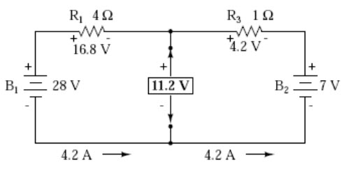
Fig. 9.5

The voltage between the two load connection points can be figured from the one of the battery’s voltage and one of the resistor’s voltage drops, and comes out to 11.2 volts. This is our “Thevenin voltage” (EThevenin) in the equivalent circuit:

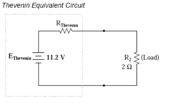
Fig. 9.6

To find the Thevenin series resistance for our equivalent circuit, we need to take the original circuit (with the load resistor still removed), remove the power sources (in the same style as we did with the Superposition Theorem: voltage sources replaced with wires and current sources replaced with breaks), and figure the resistance from one load terminal to the other:

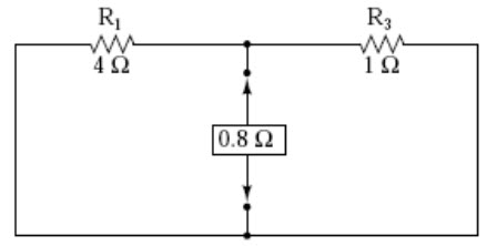
Fig. 9.7

With the removal of the two batteries, the total resistance measured at this location is equal to R1 and R3 in parallel: 0.8. This is our “Thevenin resistance” (R_Thevenin) for the equivalent circuit:

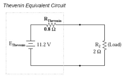
Fig.9.8

With the load resistor (2) attached between the connection points, we can determine voltage across it and current through it as though the whole network were nothing more than a simple series circuit:

	RThevenin	RLoad	Total
E	3.2	8	11.2	Volts
I	4	4	4	Amps
R	0.8	2	2.8	Ohms

 Notice that the voltage and current figures for R2 (8 volts, 4 amps) are identical to those found using other methods of analysis. Also notice that the voltage and current figures for the Thevenin series resistance and the Thevenin source (total) do not apply to any component in the original, complex circuit. Thevenin’s Theorem is only useful for determining what happens to a single resistor in a network: the load. The advantage, of course, is that you can quickly determine what would happen to that single resistor if it were of a value other than 2 without having to go through a lot of analysis again. Just plug in that other value for the load resistor into the Thevenin equivalent circuit and a little bit of series circuit calculation will give you the result.

REVIEW:

Thevenin’s Theorem is a way to reduce a network to an equivalent circuit composed of a single voltage source, series resistance, and series load. Steps to follow for Thevenin’s Theorem:

• Find the Thevenin source voltage by removing the load resistor from the original circuit and calculating voltage across the open connection points where the load resistor used to be.

• Find the Thevenin resistance by removing all power sources in the original circuit (voltage sources shorted and current sources open) and calculating total resistance between the open connection points.

• Draw the Thevenin equivalent circuit, with the Thevenin voltage source in series with the Thevenin resistance. The load resistor re-attaches between the two open points of the equivalent circuit.

• Analyze voltage and current for the load resistor following the rules for series circuits.

Norton’s Theorem

Norton’s Theorem states that it is possible to simplify any linear circuit, no matter how complex, to an equivalent circuit with just a single current source and parallel resistance connected to a load. Just as with Thevenin’s Theorem, the qualification of “linear” is identical to that found in the Superposition Theorem: all underlying equations must be linear (no exponents or roots).

Contrasting our original example circuit (fig.9.9) against the Norton equivalent: it looks something like this:

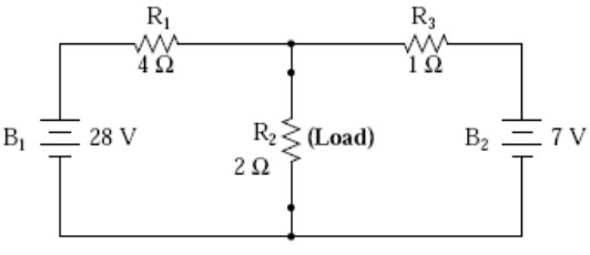
 Fig. 9.9

. . . after Norton conversion (fig.9.10) . . .

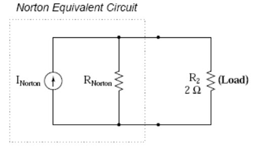
Fig. 9.10

Remember that a current source is a component whose job is to provide a constant amount of current, outputting as much or as little voltage necessary to maintain that constant current. As with Thevenin’s Theorem, everything in the original circuit except the load resistance has been reduced to an equivalent circuit that is simpler to analyze. Also similar to Thevenin’s Theorem are the steps used in Norton’s Theorem to calculate the Norton source current (I_Norton) and Norton resistance (R_Norton). As before, the first step is to identify the load resistance and remove it from the original circuit (fig.9.11).

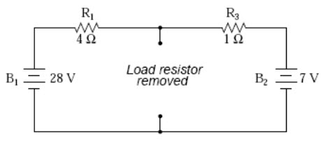Fig. 9.11

Then, to find the Norton current (for the current source in the Norton equivalent circuit), place a direct wire (short) connection between the load points and determine the resultant current. Note that this step is exactly opposite the respective step in Thevenin’s Theorem, where we replaced the load resistor with a break (open circuit fig.9.12).

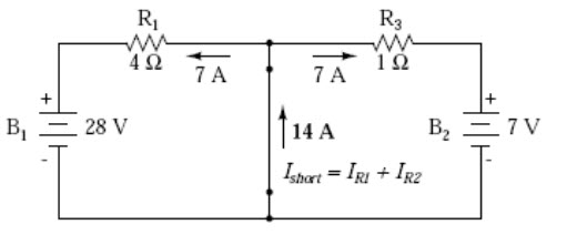
Fig. 9.12

With zero voltage dropped between the load resistor connection points, the current through R1 is strictly a function of B1’s voltage and R1’s resistance: 7 amps (I=E/R). Likewise, the current through R3 is now strictly a function of B2’s voltage and R3’s resistance: 7 amps (I=E/R). The total current through the short between the load connection points is the sum of these two currents: 7 amps + 7 amps = 14 amps. This figure of 14 amps becomes the Norton source current (I_Norton) in our equivalent circuit (fig.9.13).

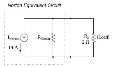
Fig. 9.13

Remember, the arrow notation for a current source points in the direction opposite that of electron flow. Again, apologies for the confusion. For better or for worse, this is standard electronic symbol notation. Blame Mr. Franklin again! To calculate the Norton resistance (R_Norton), we do the exact same thing as we did for calculating Thevenin resistance (R_Thevenin): take the original circuit (with the load resistor still removed), remove the power sources (in the same style as we did with the Superposition Theorem: voltage sources replaced with wires and current sources replaced with breaks), and figure total resistance from one load connection point to the other (fig.9.14).

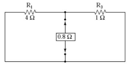
Fig. 9.14

Now our Norton equivalent circuit looks like this (fig.9.15)

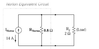
Fig. 9.15

If we re-connect our original load resistance of 2, we can analyze the Norton circuit as a simple parallel arrangement:

	RNortan	RLoad	Total
E	8	8	8	Volts
I	10	4	14	Amps
R	0.8	2	571.43m	Ohms

 

As with the Thevenin equivalent circuit, the only useful information from this analysis is the voltage and current values for R2; the rest of the information is irrelevant to the original circuit. However, the same advantages seen with Thevenin’s Theorem apply to Norton’s as well: if we wish to analyze load resistor voltage and current over several different values of load resistance, we can use the Norton equivalent circuit again and again, applying nothing more complex than simple parallel circuit analysis to determine what’s happening with each trial load.

REVIEW:

Norton’s Theorem is a way to reduce a network to an equivalent circuit composed of a single current source, parallel resistance, and parallel load. Steps to follow for Norton’s Theorem:

• Find the Norton source current by removing the load resistor from the original circuit and calculating current through a short (wire) jumping across the open connection points where the load resistor used to be.

• Find the Norton resistance by removing all power sources in the original circuit (voltage sources shorted and current sources open) and calculating total resistance between the open connection points.

• Draw the Norton equivalent circuit, with the Norton current source in parallel with the Norton resistance. The load resistor re-attaches between the two open points of the equivalent circuit.

• Analyze voltage and current for the load resistor following the rules for parallel circuit