Electrical Circuits 3(2+1)

LESSON 15. Sinusoidal Response of R-L & R-C Circuit

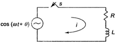
Fig.15.1

\[V\,\cos \,\left( {\omega t + \theta } \right)=Ri + L{{di} \over {dt}}...................................................\left( {15.1} \right)\]

\[{{di} \over {dt}} + {R \over L}i={V \over L}\,\,\cos \,\left( {\omega t + \theta } \right)\]

The corresponding characteristic equation is

\[\left( {D + {R \over L}} \right)i={{} \over L}\,\cos \,\left( {\omega t + \theta } \right)...................................................\left( {15.2} \right)\]

For the above equation, the solution consists of two parts, viz. complementary function and particular integral.

The complementary function of the solution i is

\[{i_c}=c{e^{ - t\left( {R/L} \right)}}...................................................\left( {15.3} \right)\]

The particular solution can be obtained by using undetermined co-efficient.

By assuming \[{i_p}=A\,\cos \,\left( {\omega t + \theta } \right) + B\,\,\sin \,\left( {\omega t + \theta } \right)...................................................\left( {15.4} \right)\]

\[i_p^'=A\omega \,\sin \,\left( {\omega t + \theta } \right) + B\omega \,\cos \,\left( {\omega t + \theta } \right)...................................................\left( {15.5} \right)\]

Substituting Eqs. 15.4 and 15.5 in Eq.15.2, we have

\[\left\{ { - A\omega \,\sin \,\left( {\omega t + \theta } \right) + \,B\omega \,\cos \left( {\omega t + } \right)} \right\} + {R \over L}\left\{ {A\,\cos \,\left( {\omega t + \theta } \right) + B\,\,\sin \,\,\left( {\omega t + \theta } \right)} \right\}={V \over L}\cos \,\left( {\omega t + \theta } \right)\]

or \[\left({ - A\omega + {{BR} \over L}} \right)\,\sin \,\left({\omega t+\theta}\right) + \left({B\omega + {{AR}\over L}}\right)\,\cos \,\,\left( {\omega t + \theta }\right)={V \over L}\,\cos \,\left({\omega t + \theta }\right)\]

Comparing cosine terms and sine terms, we get

\[-A\omega+{{BR}\over L}=0\]

\[B\omega+{{AR} \over L}={V \over L}\]

From the above equations, we have

\[A=V{R \over {{R^2} + {{\left( {\omega L} \right)}^2}}}\]

\[B=V{{\omega L} \over {{R^2} + {{\left( {\omega L} \right)}^2}}}\]

Substituting the values of A and B in Eq.11.20, we get

\[{i_p}=V{R \over {{R^2} + {{\left( {\omega L} \right)}^2}}}\cos \,\left( {\omega t + \theta } \right) + V{{\omega L} \over {{R^2} + {{\left( {\omega L} \right)}^2}}}\,\sin \,\left( {\omega t + \theta } \right)...................................................\left( {15.6} \right)\]

Putting \[M\,\cos\,\phi={{VR}\over{{R^2}+{{\left({\omega L}\right)}^2}}}\]

\[M\,\sin\,\phi=\,V{{\omega L}\over{{R^2}+{{\left({\omega L} \right)}^2}}}\]

to find M and ø, we divide one equation by the other

\[{{M\,\sin \,\phi} \over {M\,\cos \,\phi}}=\,\tan \,\phi \,=\,{{\omega L} \over R}\,\]

Squaring both equation and adding, we get

\[{M^2}\,{\cos ^2}\,\phi+{M^2}\,{\sin ^2}\,\phi={{{V^2}} \over {{R^2} + {{\left( {\omega L} \right)}^2}}}\]

or \[M={V \over {\sqrt {{R^2} + {{\left( {\omega L} \right)}^2}} }}\]

The particular current becomes

\[{i_p}={V\over{\sqrt{{R_2}+{{\left({\omega L}\right)}^2}}}}\,\cos\,\left({\omega t+\theta-{{\tan}^{-1}}{{\omega L}\over R}} \right)...................................................\left( {15.7} \right)\]

The complete solution for the current \[i={i_c} + {i_p}\]

\[i=c{e^{-t\left({R/L} \right)}} + {V \over{\sqrt{{R^2} + {{\left({\omega L} \right)}^2}}}}\,\cos \,\left({\omega t + \theta -{{\tan }^{-1}}{{\omega L} \over R}} \right)\]

Since the inductor does not allow sudden changes in currens, at t=0, i=o

\[c=-{V \over{\sqrt{{R^2} + {{\left( {\omega L}\right)}^2}} }}\,\,\cos \,\,\left( {\theta-{{\tan }^{-1}}{{\omega L}\over R}} \right)\]

The complete solution for the current is

\[i=\,{e^{-\left( {R/L} \right)t}}\left[ {{{-V} \over {\sqrt{{R^2} + {{\left( {\omega L} \right)}^2}} }}\,\,\cos \,\,\left({\theta-{{\tan }^{-1}}{{\omega L} \over R}} \right)} \right]\]

\[+{V \over{\sqrt{{R^2}+{{\left( {\omega L} \right)}^2}} }}\,\,\cos \,\,\left( {\omega t +\theta-{{\tan }^{-1}}{{\omega L}\over R}}\right)\]

15.2. Sinusoidal Response of R-C Circuit

Consider a circuit consisting of resistance and capacitance in series as shown in Fig.15.2.  The switch, S, is closed at t=0.  At t=0, a sinusoidal voltage V cos (wt+q) is applied to the R-C circuit, where V is the amplitude of the wave and q is the phase angle.  Applying Kirchhoff’s voltage law to the circuit results in the following differential equation.

\[V\,\cos \,\left( {\omega t + \theta } \right) = Ri + {1 \over C}\int {idt} ...................................................\left( {15.8} \right)\]

\[R{{di} \over {dt}} + {i \over C}=-V\,\,\omega \,\sin \,\left( {\omega t + \theta } \right)\]

\[\left( {D + {1 \over {RC}}i=-{{V\omega } \over R}\,\sin \,\left( {\omega t + \theta } \right)} \right)...................................................\left( {15.9} \right)\]

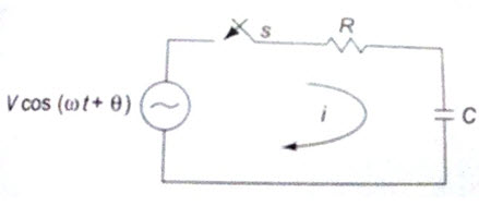
Fig. 15.2

The complementary function i_c = ce^-t/RC \[...................................................\left( {15.10} \right)\]

The particular solution can be obtained by using undermined coefficients.

\[{i_p}=A\,\cos \,\left( {\omega t + \theta } \right) + B\,\sin \,\left( {\omega t + \theta } \right)...................................................\left( {15.11} \right)\]

\[i_p^'=A\omega \,\sin \,\left( {\omega t + \theta } \right) + B\omega \,\cos \,\left( {\omega t + \theta } \right)...................................................\left( {15.12} \right)\]

Substituting Eqs. 15.11 and 15.12 in Eq. 15.9, we get

\[\left\{ { - A\omega \,\sin \,\left( {\omega t + \theta } \right) + B\omega \,\cos \,\left( {\omega t + \theta } \right)} \right\} + {1 \over {RC}}\left\{ {A\,\cos \,\left( {\omega t + \theta } \right) + B\,\sin \,\left( {\omega t + \theta } \right)} \right\}\]

\[=-{{V\omega } \over {R\,}}\,\sin \,\left( {\omega t + \theta } \right)\]

Comparing both sides, \[-A\omega+{B\over{RC}}=-{{V\omega}\over R}\]

\[B\omega+{A\over{RC}}=0\]

From which,

\[A = \frac{{VR}}{{{R^2} + {{\left( {\frac{1}{{\omega c}}} \right)}^2}}}\]

and \[B = \frac{{ - V}}{{\omega C\left[ {{R^2} + {{\left( {\frac{1}{{\omega c}}} \right)}^2}} \right]}}\]

Substituting the values of A and B in Eq. 15.11, we have

\[{i_p} = \frac{{VR}}{{{R^2}+{{\left( {\frac{1}{{\omega c}}}\right)}^2}}}\,\cos\;\,\left( {\omega t+\theta }\right)+\frac{{-V}}{{\omega C\left[ {{R^2}+{{\left( {\frac{1}{{\omega C}}}\right)}^2}}\right]}}\,\sin\,\left( {\omega t+\theta } \right)\]

Putting \[M\,\cos\,\varphi=\frac{{VR}}{{{R^2}+{{\left({\frac{1}{{\omega C}}}\right)}^2}}}\]

and \[M\,\sin\,\varphi =\frac{V}{{\omega C\left[{{R^2}+{{\left( {\frac{1}{{\omega C}}}\right)}^2}}\right]}}\]

To find M and ø, we divide one equation by the other,

\[{{M\,\sin \,\phi } \over {M\,\cos \,\phi }}=\tan \,\phi={1 \over {\omega CR}}\]

Squaring both equations and adding, we get

\[{M^2}\,{\cos ^2}\,\varphi +{M^2}\,{\sin ^2}\,\varphi =\frac{{{V^2}}}{{\left[{{R^2}+{{\left({\frac{1}{{\omega C}}}\right)}^2}}\right]}}\]

\[M =\frac{V}{{\sqrt{{R^2}+{{\left({\frac{1}{{\omega C}}}\right)}^2}}}}\]

The particular current becomes

\[{i_p}=\frac{V}{{{R^2}+{{\left({\frac{1}{{\omega c}}}\right)}^2}}}\,\cos\;\left({\omega t+\theta+{{\tan}^{-1}}\frac{1}{{\omega CR}}}\right)...................................................\left( {15.13} \right)\]

The complete solution for the current i=i_c+i_p

\[{i_p}=c{e^{-\left({t/RC}\right)}}+\frac{V}{{{R^2}+{{\left({\frac{1}{{\omega c}}}\right)}^2}}}\,\cos\;\left({\omega t+\theta+{{\tan}^{-1}}\frac{1}{{\omega CR}}}\right)...................................................\left( {15.14} \right)\]

Since the capacitor does not allow sudden changes in voltages at \[t=0,\,i={V \over R}\cos \,\theta\]

\[c=\frac{V}{R}\cos\,\theta-\frac{V}{{\sqrt{{R^2}+{{\left({\frac{1}{{\omega C}}}\right)}^2}}}}\cos\left({\theta+{{\tan }^{-1}}\frac{1}{{\omega CR}}}\right)\]

\[c=\frac{V}{R}\cos\,\theta-\frac{V}{{\sqrt{{R^2}+{{\left({\frac{1}{{\omega C}}}\right)}^2}}}}\cos\left({\theta+{{\tan}^{-1}}\frac{1}{{\omega CR}}}\right)\]

The complete solution for the current is

\[i = e-\left({t/RC}\right)\left[{\frac{V}{R}\cos \,\theta-\frac{V}{{\sqrt{{R^2}+{{\left({\frac{1}{{\omega C}}}\right)}^2}}}}\cos\,\left({\theta+{{\tan}^{-1}}\frac{1}{{\omega CR}}}\right)}\right]\]

\[+\frac{V}{{\sqrt{{R^2}+{{\left({\frac{1}{{\omega C}}}\right)}^2}} }}\cos\,\left({\omega t+\theta+{{\tan}^{-1}}\frac{1}{{\omega CR}}}\right)...................................................\left( {15.15} \right)\]