Crop Process Engineering

Lesson 17. Theory Of Mixing

17.1 Theory of solid mixing

 As opposed to mixing of miscible liquids, the mixing of particles is often a readily reversible process. A mixture of miscible liquids leaving a mixing unit retains or even improves its mixedness during the transport process, while a well-mixed batch of particles can be separated almost completely at a subsequent process stage. Particles change their relative positions in response to movement and the subsequent rearrangement maybe more random. Powder mixing occurs when any particle changes its path of circulation. Three mechanisms have been recognized in solids mixing: convection, diffusion, and shear. In any particular process one or more of these three basic mechanisms may be responsible for the course of the operation. Other mechanisms such as segregation can also be involved during particle motions. Depending on the equipment used, mixing mechanisms can receive other classifications that will be mentioned further in this section.

 17.1.1 Convective, Diffusive and Shear Mixing

 During convective mixing, masses or groups of particles transfer together from one location to another, while in diffusion mixing, individual particles are randomly distributed over a surface developed within the mixture. In shear mixing, groups of particles are mixed through the formation of slipping planes developed within the mass of the mixture. Shear mixing is sometimes considered as part of the convective mechanism.

 In convective mixing, a circulating flow of powders is usually caused by the rotational motion of a mixer vessel, an agitating impeller (such as a ribbon or a paddle), or gas flow. This circulating flow contributes mainly to a macroscopic mixing of bulk powder mixtures. Large portions of the total mix are moved at relatively high rates, and changes at a microscopic scale are not expected. Therefore, pure convection tends to be less effective, leading to a final mixture, which may still exhibit poor mixing characteristics on a fine scale. Convective mixing is beneficial for batch mode operations but gives unfavourable effects for continuous mode mixing.

 Diffusive mixing (or random wall phenomenon) is caused by the random motion of powder particles. The rate of mixing by this mechanism is low compared with convective mixing, but diffusive mixing is essential for microscopic homogenization. It has been concluded that diffusion is the best mechanism for axial mixing, similar to diffusion of particles in gas and liquid phases. Pure diffusion, when feasible, is highly effective, producing very intimate mixtures at the level of individual particles but at an exceedingly slow rate. A trough mixer with a ribbon spiral can give almost pure convective mixing, while a simple barrel mixer gives mainly a form of diffusion mixing. These features of diffusion and convective mixing mechanisms suggest that an effective operation may be achieved by combining both, in order to take advantage of the speed of convection and the effectiveness of diffusion.

 Shear mixing is induced by the momentum exchange of powder particles having different velocities (differential velocity distribution). Shear mixing is developed by the formation of slipping planes in the bulk material; the originally coherent particle groups are gradually broken along these planes. The velocity distribution develops around the agitating impeller and the vessel walls due to compression and extension of bulk powders. It is also developed in the powder layer in rotary vessel mixers and at blowing ports in gas-flow mixers. Shear mixing can enhance semi-microscopic mixing and be beneficial in both batch and continuous operations. In free-flowing powders, both diffusive mixing and shear mixing give rise to size segregation (or de-mixing), therefore, for such powders, convective mixing is the major mechanism promoting mixing.

 Powder mixing proceeds in a mixer where the three mechanisms described above take place simultaneously. The characteristic curve of mixing is the plot of the degree of mixedness M (on a logarithmic scale) against the mixing time t (on a linear scale). The mixing time is the time measured from the start of mixing in a batch mode operation, whereas it corresponds to the mean residence time (the powder volume in a mixer divided by its volumetric flow rate) in a continuous operation. The characteristic curve of mixing is useful for the performance evaluation of mixers. Fig. 5.1 shows a schematic example of the curve, where the standard deviation is plotted on a logarithmic scale.

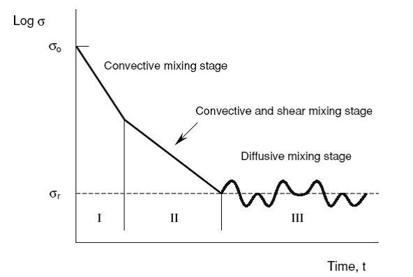
Convective mixing is dominant in the initial stage (I) and the mixing proceeds steadily by both convective and shear mechanisms in the intermediate stage (II). In the final stage (III), the effect of diffusive mixing appears and the dynamic equilibrium between mixing and segregation is reached. The degree of mixedness at this state is called the final degree of mixedness, M_∞. Various powder mixers exhibit a variety of patterns in the characteristic curve of mixing. Operating conditions and powder properties significantly influence the value of M_∞. In comparison with fluid mixing, in which diffusion can be normally regarded as spontaneous, particulate systems will only diffuse as a result of mechanical movement provided by gravity, shaking, tumbling, vibration, or any other mechanical mean. Lacey (1954) tried to adjust Fick’s equation, the simplest model for molecular diffusion in liquids, to the mixing of solids. Fick’s equation has the following form:

\[{{\partial C}\over{\partial t}}=D{{\partial ^2 C} \over {\partial x^2 }}\]...............................................(16.1)

where, C is the concentration of solids, D is the diffusivity, and x is the distance in the direction of dispersion. It is clear that the diffusivity D in solids does not have the same physical meaning as in liquids, given that D varies with the magnitude and direction of the force impelled to the powder bulk to generate movement. However, the model could describe a binary mixture of particles with the same mean diameter fed into rotating horizontal drum in such a way that a thin layer is perpendicular to the axis of rotation. The equation can be solved as a function of the number of revolutions of the mixer and the distance from one of the sidewalls. The movement of particles during a mixing operation, however, can also result in another mechanism that may retard, or even reverse, the mixing process, known as segregation.

Degree of Mixedness

 Based on a diffusive mixing mechanism and employing a modified Fick’s diffusion equation, Rose (1970) proposed the following mixing rate equation to describe the process in which both mixing and de-mixing (i.e., segregation) occur simultaneously in a mixer.

\[{{dM} \over {dt}} = A\left( {1 - M} \right) - B\lambda \] .........................................................................(16.2)

Where, A and B are mixing and de-mixing rate constants respectively

 M is the degree of mixedness and defined as;

\[M =1- {\sigma\over{\sigma o}}\]........................................................................................................(16.2.1)
Where, σ is the standard deviation

            σ₀ is the standard deviation at t=0 and

\[\lambda = \pm \sqrt {1 - M}\]...............................................................................................................(16.2.2)