Drying and Storage Engineering

Lesson 8. Theory of Diffusion

Temperature, through its effect on the saturation vapor density of air and the vapor pressure of water, determines the concentration of water molecules in the subsurface of food. Changing temperatures may create a positive, negative, or identically zero concentration gradient with respect to the vapor density in the atmosphere. If a gradient of concentration exists, there will be a net flux of water molecules down the gradient, resulting in a net growth or depletion of the subsurface water with time, even under isobaric conditions. The magnitude of this flux depends both on the magnitude of the concentration gradient and on the diffusive properties of the food product, as represented by the diffusion coefficient, D.

In the analysis of falling rate drying period, a simple diffusion model based on Fick’s second law of diffusion was considered for the evaluation of moisture transport, which is given by the following equation.

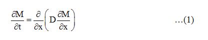
where, M is the free moisture content (kg water/kg dry matter), t is time (s), x is diffusion path or length (m) and  D is moisture dependent diffusivity (m²/s).

The diffusivity varies considerably with moisture content of the food and was estimated by analyzing the drying data using the “method of slopes” technique (Karathanos et al., 1990).

For an infinite slab being dried from both sides and with the assumptions of (i) uniform initial moisture distribution throughout the mass of the sample and (ii) negligible external resistance to mass transfer, the following initial and boundary conditions were fixed for a solution of Eqn. 1

M = M₀ at t = 0 for all L

M = M_s = M_e at t > 0, x = ± L/2 at the surface

where, M₀ is the initial moisture content; M_s is the moisture content at the surface; M_e is the equilibrium moisture content and L is the thickness of the slab.

The solution of Eqn. 3.12 for constant moisture diffusivity (D) in an infinite slab is given by Eqn. 3.13

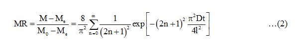
where, l is half thickness of slab.

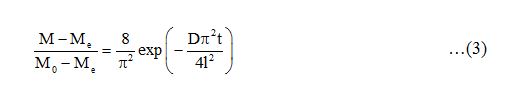
When the drying time becomes large and n > 1, Eqn. 2 can be reduced to the following form after neglecting all other terms of right hand side except the first one.

For infinite slab

 

The equation 3 is evaluated numerically for Fourier number (F₀= D.t / l²).

It is noted here that the diffusivity calculated would be a lumped value called apparent moisture diffusivity (D_a) incorporating factors that were not considered separately but would affect the drying characteristics. During microwave vacuum drying, moisture transport takes place by one or more combinations of the liquid diffusion, vapor diffusion, internal evaporation by microwaves and surface diffusion. Since the exact mechanism of moisture transport is not known, an apparent diffusivity, D_a, instead of the true diffusivity, is considered in equation 3 Therefore, the above equation is simply a model with empirical values for apparent diffusivity and not true diffusivity.

Even though the process in each test is assumed to be isothermal, experiments were conducted at four temperature levels to determine temperature dependence, which is usually assumed to follow the Arrhenius relationship which is given below:

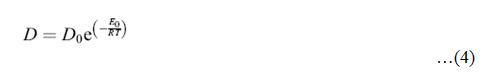
In this expression D₀ is the Arrhenius factor (m²/s), E₀ is the activation energy for moisture diffusion (kJ/mol), R is the ideal gas constant (kJ mol^-1 K^-1) and T is the sample temperature (K).

8.2 Modeling water and solid diffusion using transient solution of Fick’s law of diffusion 

The mathematical models used to describe mass transfer during osmotic dehydration are usually based upon various solutions to Fick’s Law of Diffusion. The solution applies to unsteady one dimensional transfer between a plane sheet and a well stirred solution with a constant surface concentration, that is, infinite or semi-infinite medium. The following Fick’s unsteady state diffusion model (Eqn. 3.5) can be applied to describe the osmosis mechanism:

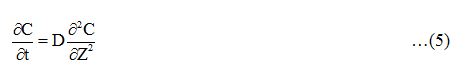
The effective diffusivity can be determined by solving the above Fick’s diffusion model using Newton Raphson method and Crank–Nicholson method (Singh et al., 2006). There are some analytical solutions of Eqn. 5 and are given by Crank (1975) for several geometries and boundary conditions. With the uniform initial water and solute concentration, the boundary conditions for a negligible external resistance and varying bulk solution concentration with the time, analytical solution of Fick’s equation for infinite slab geometry being placed in a stirred solution of limited volume is given below by Eqns. 6 and 7 for moisture loss and solute gain, respectively.

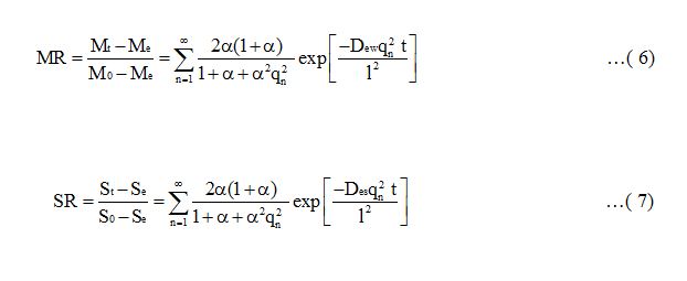
where, MR is the moisture ratio, SR is solid ratio, M_t is moisture in product at any time t (g), S_t is solids in the product at any time t (g), M_e is the equilibrium moisture in the product (g), S_e is the equilibrium solid in product (g), M₀ is the initial moisture in the product (g), S₀ is the initial solid in the product (g), D_ew is the effective water diffusivity in the product, D_es is effective solid diffusivity in the product, t  is the time of osmosis (min), l is the half thickness of the slab (m) and q_n are the non-zero positive foods of the equation:

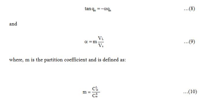
where, is volumetric solute concentration (kg of solute/m³) in solution at infinite time and  is volumetric solute concentration (kg of solute/ m³) in the product at infinite time.

Based on the model given by Crank (1975), Azuara et al. (1992) presented an expression from which the diffusion coefficient (D) can be calculated at different times during the osmotic process:

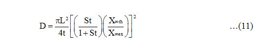
where, S is the constant related to the rate of ML or SG, X_∞th is theoretical equilibrium value for ML or SG and X_∞ex is experimental equilibrium value for ML or SG.

8.3 modeling moisture diffusivity during microwave vacuum drying

In the analysis of falling rate drying period, a simple diffusion model based on Fick’s second law of diffusion was considered for the evaluation of moisture transport, which is given by the following equation (Karathanos et al., 1990).

\[\frac{{\partial M}}{{\partial t}}=\frac{\partial}{{\partial x}}\left({D\frac{{\partial M}}{{\partial x}}}\right)\]........ (12)

where, M is the free moisture content (kg water/kg dry matter), t is time (s), x is diffusion path or length (m) and  D is moisture dependent diffusivity (m²/s).

The diffusivity varies considerably with moisture content of the food and was estimated by analyzing the drying data using the “method of slopes” technique (Karathanos et al., 1990).

For an infinite slab being dried from both sides and with the assumptions of (i) uniform initial moisture distribution throughout the mass of the sample and (ii) negligible external resistance to mass transfer, the following initial and boundary conditions were fixed for a solution of Eqn. 12

M = M₀ at t = 0 for all L

M = M_s = M_e at t > 0, x = ± L/2 at the surface

where, M₀ is the initial moisture content; M_s is the moisture content at the surface; M_e is the equilibrium moisture content and L is the thickness of the slab.

The solution of Eqn. 12 for constant moisture diffusivity (D) in an infinite slab is given by Eqn. 13

\[MR=\frac{{M-{M_e}}}{{{M_0}-{M_e}}}=\frac{8}{{{\pi^2}}}\sum\limits_{n=0}^\infty{\frac{1}{{{{\left({2n+1}\right)}^2}}}\exp \left[ {-{{\left({2n+1}\right)}^2}\frac{{{\pi ^2}Dt}}{{4{l^2}}}}\right]}\].......(13)

where, l is half thickness of slab.

When the drying time becomes large and n > 1, Eqn. 13 can be reduced to the following form after neglecting all other terms of right hand side except the first one.

For infinite slab

\[\frac{{M-{M_e}}}{{{M_0}-{M_e}}}=\frac{8}{{{\pi^2}}}\exp \left({ -\frac{{D{\pi^2}t}}{{4{l^2}}}}\right)\]..........(14)

The equation 3.13 is evaluated numerically for Fourier number (F₀= D.t / l²).

It is noted here that the diffusivity calculated would be a lumped value called apparent moisture diffusivity (D_a) incorporating factors that were not considered separately but would affect the drying characteristics.

During microwave vacuum drying, moisture transport takes place by one or more combinations of the liquid diffusion, vapor diffusion, internal evaporation by microwaves and surface diffusion. Since the exact mechanism of moisture transport is not known, an apparent diffusivity, D_a, instead of the true diffusivity, is considered in equation 14. Therefore, the above equation is simply a model with empirical values for apparent diffusivity and not true diffusivity.