Electrical Circuits 3(2+1)

LESSON 26. Series Resonance

Consider the series RLC circuit shown in Fig. 26.1.

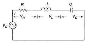
Fig. 26.1

The total impedance for the series RLC circuit is

\[Z=R + j\,\left( {X_L^{} - {X_C}} \right)\,=\,R + j\,\left( {\omega L - {1 \over {\omega C}}} \right)\]

It is clear from the circuit that the current I= V_S/Z.

The circuit is said to be in resonance if the current is in phase with the applied voltage.  In a series RLC circuit, series resonance occurs when X_L=X_C.  The frequency at which the resonance occurs is called the resonant frequency.  Since X_L=X_C, the impedance in a series RLC circuit is purely resistive.  At the resonant frequency, f_r, the voltages across capacitance and inductance are equal in magnitude.  Since they are 180⁰ out of phase with each other, they cancel each other and, hence zero voltage appears across the LC combination.

At resonance

\[{X_L}={X_C}\,\,i.e.\,\,\omega L\,=\,{1 \over {\omega C}}\]

Solving for resonant frequency, we get

\[2\pi {f_r}L\,=\,{1 \over {2\pi {f_r}C}}\]

\[f_r^2={1 \over {4{\pi ^2}LC}}\]

\[{f_r}=\,{1 \over {2\pi \sqrt {LC} }}\]

In a series RLC circuit, resonance may be produced by varying the frequency, keeping L and C constant; otherwise, resonance may be produced by varying either L or C for a fixed frequency.

26.2. Impedance and Phase Angle of a series Resonant Circuit

The impendence of a series RLC circuit is

\[\left| Z \right|\,=\,\sqrt {{R^2} + {{\left( {\omega L - {1 \over {\omega C}}} \right)}^2}}\]

The variation of X_C and X_L with frequency is shown in Fig. 26.2.

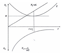
Fig.26.2

At zero frequency, both X_C and Z are infinitely large, and X_L is zero because at zero frequency the capacitor acts as an open circuit and the inductor acts as a short circuit.  As the frequency increases, X_C decreases and X_L increases.  Since X_C is larger than X_L, at frequencies below the resonant frequency \[{f_r}\] , Z decreases along with X_C. At resonant frequency \[{f_r},{X_C}={X_L},\,Z=R.\] At frequencies above the resonant frequency \[{f_r},{X_L}\] is larger than X_C, causing Z to increase.  The phase angle as a function of frequency is shown in Fig.26.3.

At a frequency below the resonant frequency, current leads the source voltage because the capacitive reactance is greater than the inductive reactance.  The phase angle decreases as the frequency approaches the resonant value, and is 0⁰ at resonance.  At frequencies above resonance, the current lags behind the source voltage, because the inductive reactance is greter than capacitive reactance. As the frequency goes higher, the phase angle approaches 90⁰.

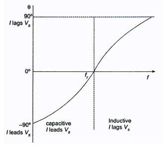
Fig.26.3

26.3. Voltages and Currents in a series resonant circuit

The variation of impedance and current with frequency is shown in Fig.26.4.

At resonant frequency, the capacitive reactance is equal to inductive reactance, and hence the impedance is minimum.  Because of minimum impedance, maximum current flows through the circuit.  The current variation with frequency is plotted.

The voltage drop across resistance, inductance and capacitance also varies with frequency.  At \[f=0\] , the capacitor acts as an open circuit and blocks current.  The complete source voltage appears across the capacitor.  As the frequency increases, X_C decreases and S_L increases, causing total reactance X_C-X_L to decrease.  As a result, the impedance decreases and the current increases. As the current increases, V_R also increases, and both V_C and V_L increase.

When the frequency reaches is resonant value \[{f_r}\]  , the impedance is equal to R, and hence, the current reaches its maximum value, and V_R is at maximum value.

As the frequency is increased above resonance, X_L-X_C to increase.  As a result continues to decrease, causing the total reactance.  As a result there is an increase in impedance and a decrease in current.  As the current decreases, V_R also decreases, and both V_C and V_L decrease. As the frequency becomes very high, the current approaches zero, both V_R and V_C approach zero, and V_L approaches V_S.

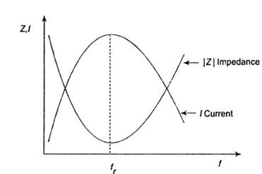Fig. 26.4

The response of different voltages with frequency is shown in Fig. 26.5

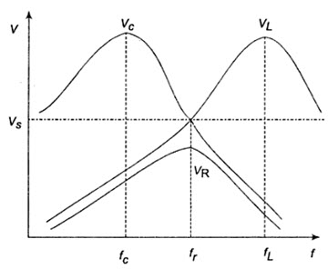
Fig. 26.5

The drop across the resistance reaches its maximum when \[f={f_r}\] .  The maximum voltage across the capacitor occurs at \[f={f_e}\] .  Similarly, the maximum voltage across the inductor occurs at \[f={f_L}\] .

\[{V_L}=I{X_L}\]

Where  \[I={V \over Z}\]

\[= \,{{\omega LV} \over {\sqrt {{R^2} + {{\left( {\omega L - {I \over {\omega C}}} \right)}^2}} }}\]

To obtain the condition for maximum voltage across the inductor, we have to take the derivative of the above equation with respect to frequency, and make it equal to zero.

\[{{d{V_L}} \over {d\omega }}=0\]

If we solve for ω, we obtain the value of ω when V_L is maximum

\[{{d{V_L}} \over {d\omega }}={d \over {d\omega }}\left\{ {\omega LV{{\left[ {{R^2} + {{\left( {\omega L - {1 \over {\omega C}}} \right)}^2}} \right]}^{ - 1/2}}} \right\}\]

\[LV{\left( {{R^2} + {\omega ^2}{L^2} - {{2L} \over C} + {1 \over {{\omega ^2}{C^2}}}} \right)^{ - 1/2}}\]

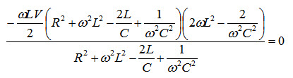
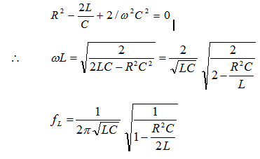
From this

Similarly, the voltage across the capacitor is

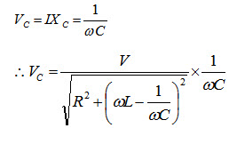
To get maximum value \[{{d{V_C}} \over {d\omega }}=0\]

If we solve for ω, we obtain the value of ω when V_C is maximum.

\[{{d{V_C}} \over {d\omega }}=\omega C{1 \over 2}{\left[ {{R^2} + {{\left( {\omega L - {1 \over {\omega C}}} \right)}^2}} \right]^{ - 1/2}}\left[ {2\left( {\omega L - {1 \over {\omega C}}} \right)\,\left( {L + {1 \over {{\omega ^2}C}}} \right)} \right]\]

       \[+ \sqrt {{R^2} + {{\left( {\omega L - {1 \over {\omega C}}} \right)}^2}\,\,C = 0}\]

From this

\[\omega _C^2\,=\,{1 \over {LC}}\, - \,{{{R^2}} \over {2L}}\]

\[{\omega _C}\,=\sqrt {{1 \over {LC}}\, - \,{{{R^2}} \over {2L}}} \,\]

\[{f_C}\,=\,{1 \over {2\pi }}\sqrt {{1 \over {LC}}\, - \,{{{R^2}} \over {2L}}} \,\]

The maximum voltage across the capacitor occurs below the resonant frequency; and the maximum voltage across the inductor occurs above the resonant frequency.

26.4. Bandwidth of an RLC Circuit

The bandwidth of any system is the range of frequencies for which the current or output voltage is equal to 70.7% of its value at the resonant frequency, and it is denoted by BW, Figure 26.6 shows the response of the series RLC circuit.

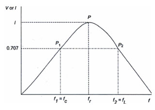
Fig. 26.6

Here the frequency \[{f_1}\] is the frequency at which the current is 0.707 times the current at resonant value, and it is called the lower cut-off frequency.  The frequency \[{f_2}\] is the frequency at which the current is 0.707 times the current at resonant value (i.e. maximum value), and is called the upper cut-off frequency.  The band width, or BW, defined as the frequency difference between \[{f_2}\,\,and\,\,{f_1}\] .

\[BW\,\,=\,\,{f_2} - {f_1}\]

The unit of BW is hertz (Hz).

If the current at P₁ is 0.707I_max, the impedance of the circuit at this point is \[\sqrt {2R,}\]  and hence

\[{1 \over {{\omega _1}C}} - {\omega _1}L = R...................................................\left( {26.1} \right)\]

Similarly,        \[{\omega _2}L - {1 \over {{\omega _2}C}} = R...................................................\left( {26.2} \right)\]

If we equate both the above equations, we get

\[{1 \over {{\omega _1}C}} - {\omega _1}L={\omega _2}L - {1 \over {{\omega _2}C}}\]

\[L\left( {{\omega _1} + {\omega _2}} \right)={1 \over C}\left( {{{{\omega _1} + {\omega _2}} \over {{\omega _1}{\omega _2}}}} \right)...................................................\left( {26.3} \right)\]

From Eq. 26.3, we get

\[{\omega _1}{\omega _2}={1 \over {LC}}\]

we have      \[\omega _r^2={1 \over {LC}}\]

\[\omega _r^2={\omega _1}{\omega _2}...................................................\left( {26.4} \right)\]

If we add Eqs 8.1 and 8.2, we get

\[{1 \over {{\omega _1}C}} - {\omega _1}L + {\omega _2}L - {1 \over {{\omega _2}C}}=2R\]

\[\left( {{\omega _2} - {\omega _1}} \right)L + {1 \over C}\left( {{{{\omega _2} - {\omega _1}} \over {{\omega _1}{\omega _2}}}} \right) = 2R...................................................\left( {26.5} \right)\]

Since \[C={1 \over {\omega _r^2L}}\]

                        and \[{\omega _1}{\omega _2}=\omega _r^2\]

\[\left( {{\omega _2} - {\omega _1}} \right)L + {{\omega _r^2\left( {{\omega _2} - {\omega _1}} \right)} \over {\omega _r^2}} = 2R...................................................\left( {26.6} \right)\]

From Eq. 26.6, we have

\[{\omega _2} - {\omega _1} = {R \over L}...................................................\left( {26.7} \right)\]

\[{f_2} - {f_1}={R \over {2\pi L}}...................................................\left( {26.8} \right)\]

or \[BW\,=\,{R \over {2\pi L}}\]

from Eq. 26.8, we have

\[{f_2} - {f_1}={R \over {2\pi L}}\]

\[{f_r} - {f_1}={R \over {4\pi L}}\]

\[\,{f_2} - {f_1}={R \over {4\pi L}}\]

The lower frequency limit \[{f_1}={f_r} - {R \over {4\pi L}}...................................................\left( {26.9} \right)\]

The upper frequency limit \[{f_2}={f_r} - {R \over {4\pi L}}...................................................\left( {26.10} \right)\]

If we divide the equation on both sides by \[{f_r}\] , we get

\[{{{f_2} - {f_1}} \over {{f_r}}}={R \over {2\pi {f_r}L}}...................................................\left( {26.11} \right)\]

Here an important property of a coil is defined.  It is the ratio of the reactance of the coil to its resistance.  This ratio is defined as the Q of the coil.  Q is known as a figure of merit, it is also called quality factor and is an indication of the quality of a coil.

\[Q{{{X_1}} \over R}={{2\pi {f_r}L} \over R}...................................................\left( {26.12} \right)\]

If we substitute Eq.26.11 in Eq.26.12, we get

\[{{{f_2} - {f_1}} \over {{f_r}}}={1 \over Q}...................................................\left( {26.13} \right)\]

The upper and lower cut-off frequencies are sometimes called the half-power frequencies.  At these frequencies the power from the source is half of the power delivered at the resonant frequency.

At resonant frequency, the power is

\[{P_{\max }}=I_{\max }^2R\]

At frequency , the power is

Similarly, at frequency \[{f_2}\] , the power is \[{P_1}={\left( {{{{I_{\max }}} \over {\sqrt 2 }}} \right)^2}\,\,R = {{I_{\max }^2R} \over 2}\]

\[{P_2}={\left( {{{{I_{\max }}} \over {\sqrt 2 }}} \right)^2}\,R\]

\[={{I_{\max }^2R} \over 2}\]

The response curve in fig.26.6 is also called the selectively curve of the circuit.  Selectivity indicates how well a resonant circuit responds to a certain frequency and eliminates all other frequencies.  The narrower the bandwidth, the greater the selectivity.

26.5. The Quality Factor (Q) and its Effect on Bandwidth

The quality factor, Q, is the ratio of the reactive power in the inductor or capacitor to the true power in the resistance in series with the coil or capacitor.

The quality factor

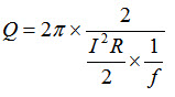
\[Q=2\pi\times {{\max imum\,energy\,\,stored} \over {energy\,\,dissipated\,per\,cycle}}\]

In an inductor, the max energy stored is given by \[{{L{I^2}} \over 2}\]

Energy dissipated per cycle = \[{\left( {{I \over {\sqrt 2 }}} \right)^2}\,\,R \times T\, = \,{{{I^2}RT} \over 2}\]

Quality factor of the coil

\[={{2\pi fL} \over R}={{\omega L} \over 2}\]

Similarly, in a capacitor, the max energy stored is given by \[{{C{V^2}} \over 2}\]

The energy dissipated per cycle   \[={\left( {I/\sqrt 2 } \right)^2}R \times T\]

The quality factor of the capacitance circuit

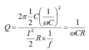
In series circuits, the quality factor \[Q={{\omega L} \over R}={1 \over {\omega CR}}\]

We have already discussed the relation between bandwidth and quality factor, which is \[Q={{{f_r}} \over {BW}}\]  .

A higher value of circuit Q results in a smaller bandwidth.  A lower value of Q causes a larger bandwidth.

26.6. Magnification in Resonance

If we assume that the voltage applied to the series RLC circuit is V, and the current at resonance is I, then the voltage across L is V_L=IX_L=(V/R) ω,L

Similarly, the voltage across C

\[{V_C} = I{X_C}={V \over {R{\omega _r}C}}\]

Since Q = 1/ω_rCR = ω_r L/R

Where w_r is the frequency at resonance.

Therefore         V_L = VQ

                                    V_C = VQ

The ratio of voltage across either L or C to the voltage applied at resonance can be defined as magnification.

Magnification = Q = V_L / V or V_C / V