Electrical Circuits 3(2+1)

LESSON 28. Classification of filters

Decibel and Neper

The attenuation of a wave filter can be expressed in decibels or nepers.  Neper is defined as the natural logarithm of the ratio of input voltage (or current) to the output voltage (or current), provided that the network is properly terminated in its characteristic impedance Z₀.

From Fig. 28.1 (a) the number of nepers, \[N={\log _e}\left[ {{{{V_1}} \over {{V_2}}}} \right]\,or\,\,{\log _e}\left[ {{{{I_1}} \over {{I_2}}}} \right]\]

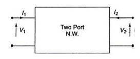
Fig. 28.1 (a)

A neper can also be expressed in terms of input power, P₁ and the output power P₂ as N = ½ log_e P₁/P₂.

A decibel is defined as en times the common logarithms of the ratio of the input power to the output power.

Decibel \[D=10\,{\log _{10}}{{{P_1}} \over {{P_2}}}\]

The decibel can be expressed in terms of the ratio of input voltage (or current) and the output voltage (or current).

\[D=10\,{\log _{10}}\left[ {{{{P_1}} \over {{P_2}}}} \right]\,\,=20\,\,{\log _{10}}\left[ {{{{I_1}} \over {{I_2}}}} \right]\]

One decibel is equal to 0.115 N.

Low Pass Filter

By definition, a low pass (LP) filter is one which passes without attenuation all frequencies up to the cut-off frequency f_c, and attenuates all other frequencies greater than ƒ_c.  The attenuation characteristic of an ideal LP filter is shown in Fig.28.1 (b).  This transmits currents of all frequencies from zero up to the cut-off frequency.  The band is called pass band or transmission band. Thus, the pass band for the LP filter is the frequency range 0 to ƒ_c.  The frequency range over which transmission does not take place is called the stop band or attenuation band.  The stop band for a LP filter is the frequency range above ƒ_c.

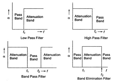
Fig.28.1 (b)

High Pass Filter

A high pass (HP) filter attenuates all frequencies below a designated cut-off frequency, ƒ_c,  and passes all frequencies above ƒ_c.  Thus the pass band of this filter is the frequency range above ƒ_c, and the stop band is the frequency range below ƒ_c.  The attenuation characteristic of a HP filter is shown in Fig.28.1 (b).

Band Pass Filter

A band pass filter passes frequencies between two designated cut-of frequencies and attenuates all other frequencies.  It is abbreviated as BP filter.  As shown in Fig.28.1 (b), a BP filter has two cut-off frequencies and will have the pass band _ƒ2 – ƒ₁; _ƒ1 is called the lower cut-off frequency, while ƒ₂ is called the upper cut-off frequency.

Band Elimination Filter

A band elimination filter passes all frequencies lying outside a certain range, while it attenuates all frequencies between the two designated frequencies.  It is also referred as band stop filter.  The characteristic of an ideal band elimination filter is shown in fig.28.1 (b).

All frequencies between _ƒ1 and ƒ₂ will be attenuated while frequencies below _ƒ1 and above ƒ₂ will be passed.

28.2. Filter Networks

Ideally a filter should have zero attenuation in the pass band.  This condition can only be satisfied if the elements of the filter are dissipation less, which cannot be realized in practice.  Filters are designed with an assumption that the elements of the filters are purely reactive.  Filters are made of symmetrical T, or p sections.  T and p sections can be considered as combinations of unsymmetrical L sections as shown in Fig.28.2.

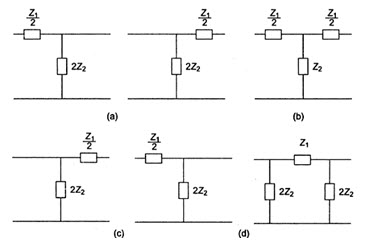
Fig.28.2

The ladder structure is one of the commonest forms of filter network.  A cascade connection of several T and \[\pi\] sections constitutes a ladder network.  A common form of the ladder network is shown in Fig.28.3.

Figure 28.3 (a) represents a T section ladder network, whereas Fig.28.3 (b) represents the \[\pi\] section ladder network. It can be observed that both networks are identical except at the ends.

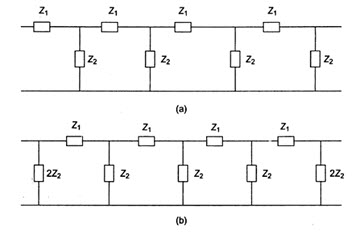
Fig. 28.3

28.3.  Equations of Filter Networks

The study of the behavior of any filter requires the calculation of its propagation constant \[\gamma\] , attenuation \[\alpha\] , phase shift β and its characteristic impedance Z₀.

T-Network

Consider a symmetrical T-network as shown in Fig.28.4

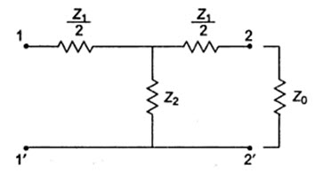
Fig.28.4

If the image impedances at port 1-1’ and port 2-2’ are equal to each other, the image impedance is then called the characteristic, or the iterative impedance, Z₀.  Thus, if the network in Fig.28.4 is terminated in Z₀, its input impedance will also be Z₀.  The value of input impedance fro the T-network when it is terminated in Z₀ is given by

                                   

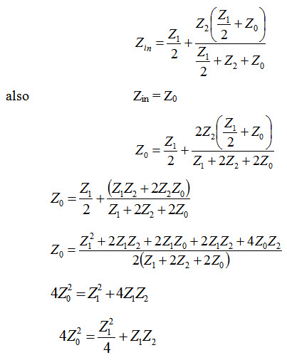
The characteristic impedance of a symmetrical T-section is

\[{Z_{0T}}=\sqrt {{{Z_1^2} \over 4} + Z_1^{}{Z_2}} ...................................................\left( {28.1} \right)\]

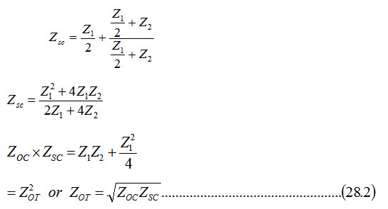
Z_0T can also be expressed in terms of open circuit impedance Z_OC and short circuit impedance Z_SC of the T-netowrk.  From Fig.17.4, the open circuit impedance \[Z_{OC}^{}={{{Z_1}} \over 2} + {Z_2}\,\,and\]

                       

Propagation Constant of T-Network

By definition the propagation constant g of the network in Fig.28.5 is given by

\[\gamma\] = log_e I₁/I₂

Writing the mesh equation for the 2^nd mesh, we get

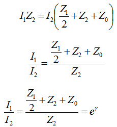
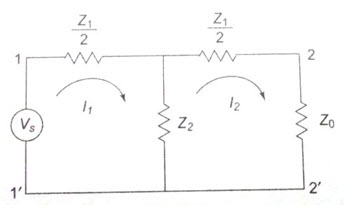
Fig.28.5

\[{{{Z_1}} \over 2} + {Z_2} + {Z_0}={Z_2}{e^\gamma }\]

\[{Z_0}={Z_2}\left( {{e^\gamma } - 1} \right) - {{{Z_1}} \over 2}...................................................\left( {28.3} \right)\]

The characteristic impedance of a T-network is given by

\[{Z_{OT}}=\sqrt {{{Z_1^2} \over 4} + {Z_1}{Z_2}} ...................................................\left( {28.4} \right)\]

Squaring Eqs. 28.3 and 28.4 and subtracting Eq.28.4 from Eq.28.3, we get

\[Z_2^2{\left( {{e^\gamma } - 1} \right)^2} + {{Z_1^2} \over 4} - {Z_1}{Z_2}\left( {{e^\gamma } - 1} \right) - {{Z_1^2} \over 4} - {Z_1}{Z_2}=0\]

\[Z_2^2{\left( {{e^\gamma } - 1} \right)^2} - {Z_1}{Z_2}\left( {1 + {e^\gamma } - 1} \right)=0\]

\[Z_2^2{\left( {{e^\gamma } - 1} \right)^2} - {Z_1}{Z_2}{e^\gamma }=0\]

\[{Z_2}{\left( {{e^\gamma } - 1} \right)^2} - {Z_1}{e^\gamma }=0\]

\[{\left( {{e^\gamma } - 1} \right)^2}={{{Z_1}{e^\gamma }} \over {{Z_2}}}\]

\[{e^\gamma } + 1 - 2{e^\gamma }={{{Z_1}} \over {{Z_2}{e^{ - \gamma }}}}\]

Rearranging the above equation, we have

\[{e^{ - \gamma }}\left( {{e^{2\gamma }} + 1 - 2{e^\gamma }} \right) = {{{Z_1}} \over {{Z_2}}}\]

\[\left( {{e^\gamma } + {e^{ - \gamma }} - 2} \right)={{{Z_1}} \over {{Z_2}}}\]

Dividing both sides by 2, we have

\[{{{e^\gamma } + {e^{ - \gamma }}} \over 2}=1 + {{{Z_1}} \over {2{Z_2}}}\]

                        Cosh \[\gamma =1 + {{{Z_1}} \over {2{Z_2}}}...................................................\left( {28.5} \right)\]

Still another expression may be obtained for the complex propagation constant in terms of the hyperbolic tangent rather than hyperbolic cosine.

\[\sinh \,\gamma=\sqrt {\cos \,{h^2}\gamma-1}\]                      

\[=\sqrt {{{\left( {1 + {{{Z_1}} \over {2{Z_2}}}} \right)}^2}}-1=\sqrt {{{{Z_1}} \over {{Z_2}}} + {{\left( {{{{Z_1}} \over {2{Z_2}}}} \right)}^2}} \]

\[Sinh\,\,\gamma=\,{1 \over {{Z_2}}}\sqrt {{Z_1}{Z_2} + {{Z_1^2} \over 4}}={{{Z_{0T}}} \over {{Z_2}}}...................................................\left( {28.6} \right)\]

Dividing by Eq.28.6 by Eq.28.5, we get

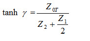
But   \[{Z_2} + {{{Z_1}} \over {{Z_2}}}={Z_{0C}}\]

Also from Eq. 28.2, \[\tanh \,\,\gamma=\sqrt {{{{Z_{sc}}} \over {{Z_{0c}}}}}\]

\[\tanh \,\,\gamma=\sqrt {{{{Z_{sc}}} \over {{Z_{oc}}}}}\]

Also     \[\sinh \,{\gamma\over 2}=\sqrt {{1 \over 2}\left( {\cosh \,\,\gamma-1} \right)}\]

Where  \[\cosh \,\,\gamma=1 + \left( {{Z_1}/2{Z_2}} \right)\]

\[=\sqrt {{{{Z_1}} \over {4{Z_2}}}} ...................................................\left( {28.7} \right)\]

\[\pi\] -Network

Consider asymmetrical p-section shown in Fig.28.6. When the network is terminated in Z₀ at port 2-2’, it input impedance is given by

                                   

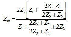
By definition of characteristic impedance, Z_in = Z₀

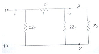
Fig.28.6

                                   

                       

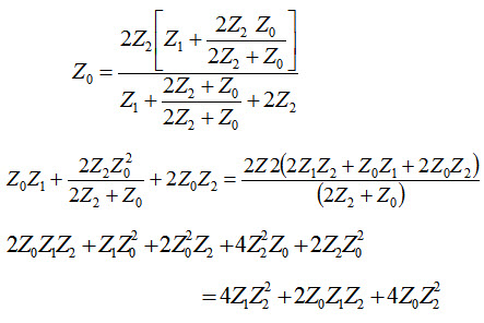
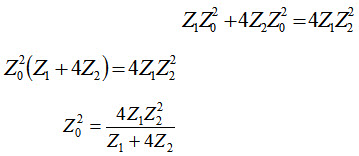
Rearranging the above equation leads to

\[{Z_0}=\sqrt {{{{Z_1}{Z_2}} \over {1 + {Z_1}/4{Z_2}}}} ...................................................\left( {28.8} \right)\]

which is the characteristic impedance of a symmetrical pnetwork,

\[{Z_{0\pi }}=\sqrt {{{{Z_1}{Z_2}} \over {{Z_1}{Z_2} + Z_1^2/4}}\]

From Eq. 28.1                        \[{Z_{OT}}=\sqrt {{{Z_1^2} \over 4} + {Z_1}{Z_2}}\]

\[{Z_{0\pi }}={{{Z_1}{Z_2}} \over {{Z_{OT}}}}...................................................\left( {28.9} \right)\]

Z_0p can be expressed in terms of the open circuit impedance Z_0c and short circuit impedance Z_SC of the p network shown in Fig.28.6 exclusive of the lead Z₀.

\[by\,\,\,\,{Z_{0C}}={{2{Z_2}\left( {{Z_1} + 2{Z_2}} \right)} \over {{Z_1} + 4{Z_2}}}\]

Similarly, the input impedance at port 1-1’ when port 2-2’ is short circuited is given by

\[{Z_{sc}}={{2{Z_1}{Z_2}} \over {2{Z_2} + {Z_1}}}\]

Hence      \[{Z_{oc}} \times {Z_{sc}}={{4{Z_1}Z_2^2} \over {{Z_1} + 4{Z_2}}} = {{{Z_1}{Z_2}} \over {1 + {Z_1}/4{Z_2}}}\]

Thus from Eq. 28.8

                              \[{Z_{0\pi }}=\sqrt {{Z_{oc}}{Z_{sc}}} ...................................................\left( {28.10} \right)\]

Propagation Constant of p-Network

The propagation constant of a symmetrical p-section is the same as that for a symmetrical T-section.

i.e.      \[\cosh \,\,\gamma=1 + {{{Z_1}} \over {2{Z_2}}}\]