Drainage Engg.

Lesson 6 Steady-State Flow to Drains

6.2   Steady-State Drainage Equations

6.2.1     Problem Definition and Assumptions

This section deals with the flow of groundwater to parallel field drains under steady-state conditions. This is a typical situation in areas with a humid climate and prolonged periods of fairly uniform, medium-intensity rainfall. The steady-state theory is based on the assumption that the rate of recharge to the aquifer is steady and that it equals the discharge of the drain. Thus, under steady-state conditions the water table position does not change as long as the recharge continues.

Fig. 6.1 shows two typical cross-sections of a drainage system under steady-state conditions. In this figure, since the aquifer receives recharge from excess rainfall, excess irrigation, or upward seepage, the water table is curved and its elevation is the highest at mid-drain spacing. For analysis, we assume the symmetry of the flow system, and hence we will consider only one half of the figure.

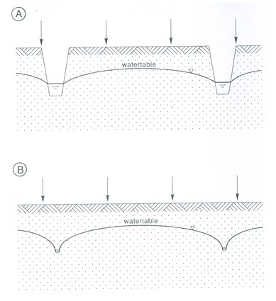
Fig. 6.1. Cross-sections of open field drains (A) and pipe drains (B), showing a curved water table under recharge.

(Source: Ritzema, 1994)

To analyze the flow of groundwater to the drainage systems, the following assumptions are made in order to simplify the complex flow process so as to apply analytical techniques:

• Subsurface flow is two-dimensional. This means that the flow is considered to be identical in any cross-section perpendicular to the drains; this is true only for infinitely long drains.

• The recharge is uniformly distributed.

• Soils are homogeneous and isotropic. Thus, spatial variation of the hydraulic conductivity within a soil layer is ignored; through soil profiles consisting of two or more layers can be handled.

Most drainage equations are based on the Dupuit-Forchheimer assumptions. These assumptions state that the streamlines in a vertical plane under study are horizontal and that the flow velocity in the plane at all depths is proportional to the slope of the water table. Based on these assumptions, the two-dimensional flow can be reduced to a one dimensional flow. Such a flow pattern is possible when the impervious layer is close to the drain. The Hooghoudt Equation (described later) is based on these conditions. If the impervious layer does not coincide with the bottom of the drain, the flow in the vicinity of the drains will be radial and the Dupuit-Forchheimer assumptions cannot be applied. Hooghoudt solved this problem by introducing an imaginary impervious layer to take into account the extra head loss caused by the radial flow. Other approximate analytical solutions were derived by Kirkham and Dagan. Kirkham (1958) presented a solution based on the potential flow theory, which takes both the flow above and below drain level into account. Dagan (1964) considered radial flow close to the drain and horizontal flow further away from it. Ernst derived a solution for a soil profile consisting of more than one soil layer.

Of the above-mentioned equations, Hooghoudt's gives the best results (Lovell and Youngs, 1984). Also, whichever equations are used to calculate drain spacings, the difference in the results will be minor in comparison with the accuracy of the input data (e.g., data on the hydraulic conductivity). Therefore, in this lesson, the Hooghoudt equation and the Ernst equation are described.

6.2.1     Hooghoudt Equation

Consider a steady-state flow to vertically-walled open drains reaching an impervious layer (Fig. 6.2). According to the Dupuit-Forchheimer assumptions, Darcy's equation can be applied to describe the flow of groundwater (q_x) through a vertical plane (y) at a distance (x) from the drainage ditch, which yields the following:

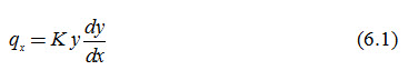
Where, q_x = unit flow rate in the x-direction (m²/day), K = hydraulic conductivity of the soil (m/day), y = height of the water table at x (m), and      = hydraulic gradient at x (dimensionless).

According to the law of conservation of mass, all the water entering the soil in the surface area midway between the drains and the vertical plane (y) at distance (x) must pass through this plane on its way to the drain. If R is the rate of recharge per unit area, then the rate of flow through the plane (y) is given as:

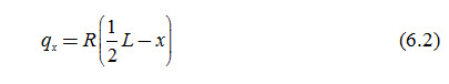
Where, R = rate of recharge per unit surface area [L/T], and L = drain spacing [L].

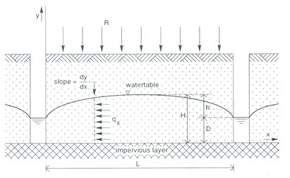
Fig. 6.2. Flow to vertically-walled drains reaching the impervious layer. (Source: Ritzema, 1994)

Since the flow in the two cases must be equal, we can equate the right sides of Eqns. (6.1) and (6.2) as follows:

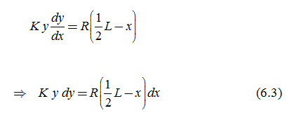
Integrating this differential equation [Eqn. (6.3)] with the lower and upper limits of x and y, we have:

 

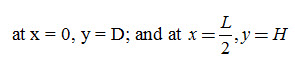
Integrating Eqn. (6.3) within these limits, we have:

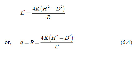
Where, D = elevation of the water level in the drain [L], H = elevation of the water table midway between the drains [L], q = drain discharge [L/T], and the remaining symbols have the same meaning as defined earlier.

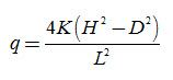
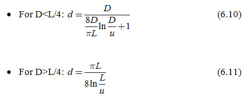
Eqn. (6.4), which was derived by Hooghoudt in 1936, is also known as the Donnan Equation (Donnan, 1946). Hooghoudt derived this equation by assuming constant and uniform rate of recharge and horizontal flow to vertical ditches. The Hooghoudt’s theory also assumes that the drains (pipe or open drains) run half full and that the drains have no entrance resistance. The second assumption (no entrance resistance) suggests that the drain is ideal. To be an ideal drain, the hydraulic conductivity of the surround (drain trench) should be at least 10 times higher than that of the undisturbed soil outside the trench (Smedema and Rycroft, 1983). If the hydraulic conductivity of the surround is less, an envelope material can be used to minimize the entrance resistance, so that a greater part of the total head could be available for flow through the soil. In case, it is not possible to use an envelope material, the entrance resistance should be introduced into the Hooghoudt equations by replacing h with (h - h_e), wherein h_e is the entrance head loss in metres. Hence, the validity of Eqn. (6.4) becomes better when the drains are of negligible width as compared to the drain spacing, shallow, fully penetrating and with a small difference between H and D such that the assumption of parallel flow is applicable. Also, homogeneous soil (constant hydraulic conductivity) is also an important pre-condition for the validity of Eqn. (6.4). Equation (6.4) can be rewritten as:

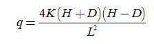
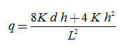
From Fig. 6.2, it is clear that H - D = h, and hence H + D = 2D + h, where h is the height of the water table above the water level in the drain. Consequently, Equation (6.4) can be written as follows:

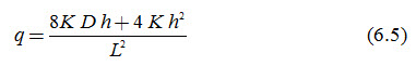
If the water level in the drain is negligible (i.e., D » 0), Eqn. (6.5) reduces to:

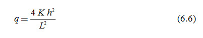
Equation (6.6) describes the flow above the drainage base (drain level)

If the impervious layer is far below drain level (D >> h), the second term in the enumerator of Eqn. (6.5) can be neglected, yielding:

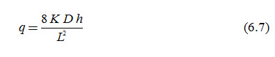
Eqn. (6.7) describes the flow below the drain level.

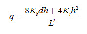
Thus, if the soil above drainage base has a different hydraulic conductivity (say K₁) than the hydraulic conductivity of the soil below drainage base (say K₂), and the drain level is at the interface between the two soil layers, Eqn. (6.5) can be written as:

 

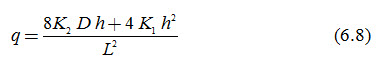
The situation of layered or stratified soil is quite common in the field. The soil above the drain level is often more permeable than that below the drain level because the soil structure above drain level gets improved by the periodic wetting and drying of the soil (resulting in the formation of cracks), and the presence of roots, micro-organisms, micro-fauna, etc.

Concept of Equivalent Depth

If the pipe or open drains do not reach the impervious layer, the flow lines will converge towards the drain and will thus no longer be horizontal (Fig. 6.3A). Consequently, the flow lines are longer (elongated) and extra head loss is required to have the same volume of water flowing into the drains. This extra head loss results in a higher water table.

Hooghoudt (1940) introduced following two simplifications in his theory to account for the extra head loss due to radial flow to the drains:

• He assumed an imaginary impervious layer above the real one, which decreases the thickness of the layer through which the water flows towards the drains.

• He treated horizontal and radial flow to pipe/tile drains as an equivalent flow to imaginary ditches with their bottoms on an imaginary impervious layer at a reduced depth.

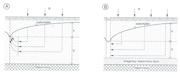
Fig. 6.3. The concept of the equivalent depth (d) to transform a combination of horizontal and radial flow shown in

(A) into an equivalent horizontal flow shown in (B). (Source: Ritzema, 1994)

Under these assumptions (Fig. 6.3B), the equivalent flow is essential horizontal, and hence  Eqn. 6.5 can be used to express the flow towards the drains, by replacing the actual depth to the impervious layer (D) with an equivalent depth (d), which is smaller than D. The equivalent depth (d) represents an imaginary thinner soil layer through which the same amount of water will flow per unit time as in the actual situation. This higher flow per unit area introduces an extra head loss, which accounts for the head loss caused by the converging flow lines. Thus, Eqn. (6.5) can be modified as follows:

Now, the only problem that remains is to find a value for the equivalent depth (d). On the basis of the method of ‘mirror images’, Hooghoudt derived a relationship between the equivalent depth (d) and, respectively, the spacing (L), the depth to the impervious layer (D), and the radius of the drain (r₀). This relationship, which is in the form of infinite series, is complex, and hence Hooghoudt prepared tables for the most common sizes of drain pipes, from which the equivalent depth (d) can be read directly. Table 6.1 (for r₀ = 0.1 m) is one such table. It is obvious from this table that the value of d increases with D until D » ¼ L. If the impervious layer is even deeper, the equivalent depth remains approximately constant; apparently the flow pattern is then no longer affected by the depth of the impervious layer.

Since the drain spacing L depends on the equivalent depth d, which in turn is a function of L, Eqn. (6.9) can only be solved by iteration. As this calculation method with the use of tables is somewhat time-consuming, Van Beers (1979) prepared nomographs from which d can be read easily.

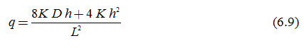
With the readily availability of computers these days, the Hooghoudt’s approximation method for calculating the equivalent depth can be replaced by exact solutions. As given below (Smedema and Rycroft, 1983):

In situations where there is no distinct impermeable layer, the depth D may be equal to the depth at which the K-value has decreased to 1/10 of the (average) K- value of the layer(s) above, provided no highly permeable layer occurs within 1-2 m below this depth (Smedema and Rycroft, 1983).

Table 6.1.Values for the equivalent depth (d) of Hooghoudt for r₀ = 0.1 m, D and L in m (after Hooghoudt, 1940)

L®	5m	7.5	10	15	20	25	30	35	40	45	50	L®	50	75	80	85	90	100	150	200	250
D												D
0.5 m	0.47	0.48	0.49	0.49	0.49	0.50	0.50	0.50	0.50	0.50	0.50	0.5	0.50	0.50	0.50	0.50	0.50	0.50	0.50	0.50	0.50
0.75	0.60	0.65	0.69	0.71	0.73	0.74	0.75	0.75	0.75	0.76	0.76	1	0.96	0.97	0.97	0.97	0.98	0.98	0.90	0.99	0.99
1.00	0.67	0.75	0.80	0.86	0.89	0.91	0.93	0.94	0.96	0.96	0.96	2	1.72	1.80	1.82	1.82	1.83	1.85	1.00	1.92	1.94
1.25	0.70	0.82	0.89	1.00	1.05	1.09	1.12	1.13	1.14	1.14	1.15	3	2.29	2.49	2.52	2.54	2.56	2.60	2.72	2.70	2.83
1.50	0.70	0.88	0.97	1.11	1.19	1.25	1.28	1.31	1.34	1.35	1.36	4	2.71	3.04	3.08	3.12	3.16	3.24	3.46	3.58	3.66
1.75	0.70	0.91	1.02	1.20	1.30	1.39	1.45	1.49	1.52	1.55	1.57	5	3.02	3.49	3.55	3.61	3.67	3.78	4.12	4.31	4.43
2.00	0.70	0.91	1.13	1.28	1.41	1.50	1.57	1.62	1.66	1.70	1.72	6	3.23	3.85	3.93	4.00	4.08	4.23	4.70	4.97	5.15
2.25	0.70	0.91	1.13	1.34	1.50	1.69	1.69	1.76	1.81	1.84	1.86	7	3.43	4.14	4.23	4.33	4.42	4.62	5.22	5.57	5.81
2.50	0.70	0.91	1.13	1.38	1.57	1.69	1.79	1.87	1.94	1.99	2.02	8	3.56	4.38	4.49	4.61	4.72	4.95	5.68	6.13	6.43
2.75	0.70	0.91	1.13	1.42	1.63	1.76	1.88	1.98	2.05	2.12	2.18	9	3.66	4.57	4.70	4.82	4.95	5.23	6.09	6.63	7.00
3.00	0.70	0.91	1.13	1.45	1.67	1.83	1.97	2.08	2.16	2.23	2.29	10	3.74	4.74	4.89	5.04	5.18	5.47	6.45	7.09	7.53
3.25	0.70	0.91	1.13	1.48	1.71	1.88	2.04	2.16	2.26	2.35	2.42	12.5	3.74	5.02	5.20	5.38	5.56	5.92	7.20	8.06	8.68
3.50	0.70	0.91	1.13	1.50	1.75	1.93	2.11	2.24	2.35	2.45	2.54	15	3.74	5.20	5.40	5.60	5.80	6.25	7.77	8.84	9.64
3.75	0.70	0.91	1.13	1.52	1.78	1.97	2.17	2.31	2.44	2.54	2.64	17.5	3.74	5.30	5.53	5.76	5.99	6.44	8.20	9.47	10.4
4.00	0.70	0.91	1.13	1.52	1.81	2.02	2.22	2.37	2.51	2.62	2.71	20	3.74	5.30	5.62	5.87	6.12	6.60	8.54	9.97	11.1
4.50	0.70	0.91	1.13	1.52	1.85	2.08	2.31	2.50	2.63	2.76	2.87	25	3.74	5.30	5.74	5.96	6.20	6.79	8.99	10.7	12.1
5.00	0.70	0.91	1.13	1.52	1.88	2.15	2.38	2.58	2.75	2.89	3.02	30	3.74	5.30	5.74	5.96	6.20	6.79	9.27	11.3	12.9
5.50	0.70	0.91	1.13	1.52	1.88	2.20	2.43	2.65	2.84	3.00	3.15	35	3.74	5.30	5.74	5.96	6.20	6.79	9.44	11.6	13.4
6.00	0.70	0.91	1.13	1.52	1.88	2.20	2.48	2.70	2.92	3.09	3.26	40	3.74	5.30	5.74	5.96	6.20	6.79	9.44	11.8	13.8
7.00	0.70	0.91	1.13	1.52	1.88	2.20	2.54	2.81	3.03	3.24	3.43	45	3.74	5.30	5.74	5.96	6.20	6.79	9.44	12.0	13.8
8.00	0.70	0.91	1.13	1.52	1.88	2.20	2.57	2.85	3.13	3.35	3.56	50	3.74	5.30	5.74	5.96	6.20	6.79	9.44	12.1	14.3
9.00	0.70	0.91	1.13	1.52	1.88	2.20	2.57	2.89	3.18	3.43	3.66	60	3.74	5.30	5.74	5.96	6.20	6.79	9.44	12.1	14.6
10.00	0.70	0.91	1.13	1.52	1.88	2.20	2.57	2.89	3.23	3.48	3.74	¥	3.88	5.38	5.76	6.00	6.26	6.82	9.55	12.2	14.7
¥	0.71	0.93	1.14	1.53	1.89	2.24	2.58	2.91	3.24	3.56	3.88

In the above equation, u is the entrance area, which is equal to the wetted perimeter of a semi-circle (i.e., pr₀). That is,

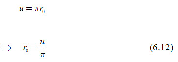
Where, r₀ = radius of the drain [L], and u = wetted perimeter of the drain [L].

For open drains, the equivalent radius (r₀) can be calculated by substituting the wetted perimeter of the open drain for u in Eqn. (6.12). For pipe drains laid in trenches, the wetted perimeter is computed as:

Where, b is the width of the trench [L].

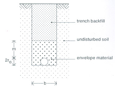
Fig. 6.4. Drain pipe with gravel envelope in the drain trench.

(Source: Ritzema, 1994)

If an envelope material is used around the pipe drain (Fig. 6.4), Eqn. (6.13) becomes:

Where, m is the height of the envelope above the drain [L], and the remaining symbols have the same meaning as defined earlier.

6.2.3     Ernst Equation

The Hooghoudt Equation can be applied for a homogeneous soil profile or for a two-layered soil profile provided that the interface between the two layers coincides with the drain level. In contrast, the Ernst Equation is applicable to any type of two-layered soil profile. It has an advantage over the Hooghoudt Equation that the interface between the two layers can be either above or below drain level. It is especially useful when the top soil layer has a considerably lower hydraulic conductivity than the bottom soil layer.

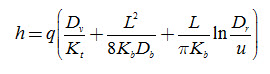
To obtain a generally applicable solution for soil profiles consisting of layers with different hydraulic conductivities, Ernst (1956; 1962) divided the flow to the drains into vertical, horizontal, and radial components (Fig. 6.5). The extent of the three flow zones differs from case to case, depending mainly on the relative magnitude of h, L and D. Consequently, the total available head (h) can be visualized as being made up of the head loss due to vertical flow (h_v), horizontal flow (h_h), radial flow (h_r), and entry flow (h_e):

 

Generally, h_e is assumed to be zero (ideal drains).

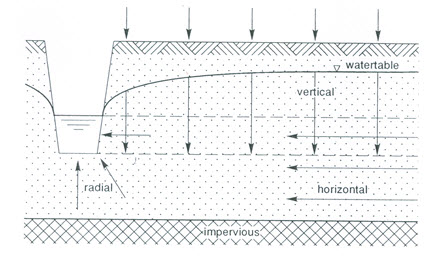
Fig. 6.5. Geometry of two-dimensional flow towards drains according to Ernst.

(Source: Ritzema, 1994)

(i) Vertical Flow

Vertical flow is usually assumed to take place in the zone between the water table and the drain level (Fig. 6.5); though in reality it often goes deeper. The head loss due to a vertical flow of q through a soil layer of thickness D_v and a vertical hydraulic conductivity of K_v can be calculated by applying Darcy’s Law:

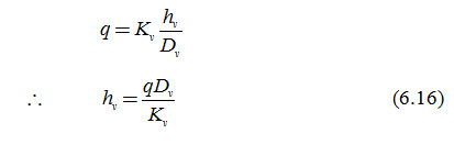
Where, h_v = head loss due to vertical flow [L].

As the vertical hydraulic conductivity is difficult to measure under field conditions, it is often replaced with the horizontal hydraulic conductivity, which is rather easy to measure by the auger-hole method. In principle, this is not correct, especially not in the alluvial soils where big differences between horizontal and vertical conductivity may occur. The vertical head loss, however, is generally small compared to the horizontal and radial head losses. Therefore, the error caused by replacement of K_v with K_h can be neglected.

(ii) Horizontal Flow

The horizontal flow is assumed to take place below drain level (Fig. 6.5). Analogous to Eqn. (6.7), the horizontal head loss (h_h) can be expressed as:

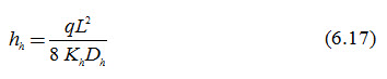
Where, K_h D_h = transmissivity of the soil layers through which the water flows horizontally [L²/T], and the remaining symbols have the same meaning as defined earlier.

If the impervious layer is very deep, the value of K_h D_h increases to infinity and hence the horizontal head loss decreases to zero. To avoid this situation, the maximum thickness of the soil layer below the drain level through which horizontal flow is considered (D_h) is restricted to ¼ L (i.e., D_h< ¼ L ).

(iii) Radial Flow

The radial flow is also assumed to take place below drain level (Fig. 6.5), because towards the end of its path the flow converges radially onto the drain. The head loss caused by the radial flow can be expressed as:

 

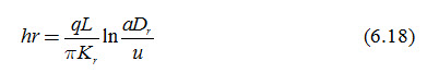
Where, K_r = radial hydraulic conductivity [L/T], a = geometry factor of the radial resistance (dimensionless), D_r = thickness of the layer in which the radial flow is considered [L], and u = wetted perimeter of the drain [L], and the remaining symbols have the same meaning as defined earlier.

Equation (6.18) has the same restriction for the depth of the impervious layer as the equation for horizontal flow (i.e., D_r < ¼ L).

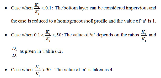
The geometry factor (a) depends on the soil profile and the position of the drain. In a homogeneous soil profile, the geometry factor equals one; in a layered soil, the geometry factor depends on whether the drains are in the top or bottom soil layer. If the drains are in the bottom layer, the radial flow is assumed to be restricted to this layer, and again a = 1. If the drains are in the top layer, the value of ‘a’ depends on the ratio of the hydraulic conductivity of the bottom (K_b) and top (K_t) layer. Using the relaxation method, Ernst (1962) distinguished the following situations:

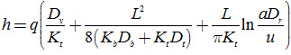
Now, the equations for the vertical head los [Eqn. (6.16)], horizontal head loss [Eqn. (6.17)], and the radial head loss [Eqn. (6.18)] can be substitute into Eqn. (6.15) to obtain the total head loss:

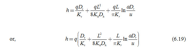
Table 6.2. The Geometry factor (a) obtained by the relaxation method (after Van Beers, 1979)

Sl. No.	Ratio	Value of ‘a’ for different Ratios
		1	2	4	8	16	32
1	1	2.0	3.0	5.0	9.0	15.0	30.0
2	2	2.4	3.2	4.6	6.2	8.0	10.0
3	3	2.6	3.3	4.5	5.5	6.8	8.0
4	5	2.8	3.5	4.4	4.8	5.6	6.2
5	10	3.2	3.6	4.2	4.5	4.8	5.0
6	20	3.6	3.7	4.0	4.2	4.4	4.6
7	50	3.8	4.0	4.0	4.0	4.2	4.6

Equation (6.19) is commonly known as the Ernst Equation. If the design discharge rate (q) and the total hydraulic head (h) are known, this quadratic equation for the drain spacing (L) can be solved directly.

Note that because of the restriction on the depth of the impervious layer in the Ernst Equation, the drain spacings calculated by this equation for deeper impervious layers are usually too small.

6.3  Selection of Suitable Steady-State  Drainage Equations

It is clear from the above discussion that two important factors to be considered for selecting the most appropriate steady-state equation are the soil profile and the relative position of the drains in the profile. Table 6.3 summarizes some of the more common field situations and appropriate equation for each of them. In all the cases, the lower boundary is formed by an impervious layer. Detailed discussion about these field situations is given in Ritzema (1994).

Table 6.3. Summary of the steady-state equations (Source: Ritzema, 1994)

Sl. No.	Soil Profile	Location of Drain	Equation
1	Homogeneous	On the top of the impervious layer	Hooghoudt/Donnan Equation:
2	Homogeneous	Above the impervious layer	Hooghoudt Equation with equivalent depth:
3	Two layers	An interface of the two soil layers	Hooghoudt Equation:
4	Two layers (Kt < Kb)	In the bottom layer	Ernst Equation:
5	Two layers (Kt < Kb)	In the top layer	Ernst Equation:     Where, Dt = Dr + ½ h, and Dv = h.

6.4   Application of Steady-State Drainage Equations

To calculate the drain spacing with steady-state equations, we must have information on the soil characteristics, the agricultural design criteria, and the technical criteria. The required soil data include a description of the soil profile, the depth of the impervious layer, and the hydraulic conductivity.

The agricultural design criteria are the required depth of the water table (h) and the corresponding design discharge (q). They depend on many factors (e.g., type of crop, and climate). The ratio q/h is sometimes called the drainage criterion or drainage intensity. The higher the q/h ratio, the more safety is built into the drainage system to prevent high water tables. The use of the steady-state equations discussed in the previous section is demonstrated through one example given below.

6.4.1 Example Problem (after Ritzema, 1994)

In an agricultural area, high water table condition occurs. A subsurface drainage system is to be installed to control the water table under the following conditions:

(1) Agricultural drainage criteria:

• Design discharge rate is 1 mm/day

• The depth of the water table midway between the drains is to be kept at 1.0 m below the soil surface.

(2) Technical criteria:

• Drains will be installed at a depth of 2 m;

• PVC drain pipes with a radius of 0.10 m will be used.

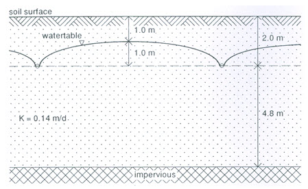
Fig. 6.6. Calculation of drain spacing in a one-layered soil profile.

(Source: Ritzema, 1994)

Field investigation revealed that there is a layer of low conductivity at 6.8 m depth, which can be regarded as the base of the flow region (Fig. 6.6). Auger-hole method was used to calculate the hydraulic conductivity of the soil above the impervious layer and its average value was found to be 0.14 m/day. Calculate the spacing of pipe drains.

Solution:

If we assume a homogeneous soil profile, we can use the Hooghoudt formula [Eqn. (6.9)] to calculate the drain spacing. We have the following data:

q = 1 mm/day = 0.001 m/day,

h = 2.0 – 1.0 = 1.0 m,

r₀ = 0.10 m,

K = 0.14 m/day, and

D = 6.8 – 2.0 = 4.8 m

Substitution of the above values into Equation (6.9) yields:

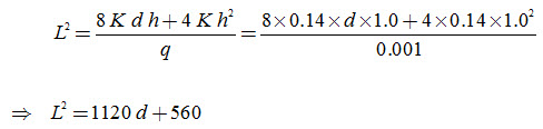
As the equivalent depth, (d) is a function of L (among other factors), we can solve this quadratic equation for L by the trial-and-error method.

First Trial: Assume L = 75 m. We can read the equivalent depth, (d) from Table 6.1.

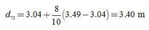
Thus, L² = 1120 ´ 3.40 + 560 = 4368 m². This is not in agreement with the assumed value of L, because L² = 75² = 5625 m². Apparently, the drain spacing of 75 m is too wide.

Second Trial: Assume L = 50 m. In this case, d is obtained from Table 6.1 as:

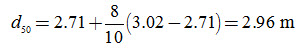
Thus, L² = 1120 ´ 2.96 + 560 = 3875 m². Again, this is not in agreement with the assumed value of L, because L² = 50² = 2500 m². Thus, a drain spacing of 50 m is very narrow.

Third Trial: Assume L = 65 m. In this case d is obtained as:

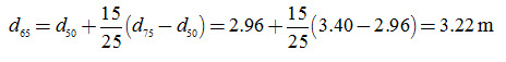
Thus, L² = 1120 ´ 3.22 + 560 = 4166 m². This is reasonably close to the assumed value of L because L² = 65² = 4225 m². Therefore, a drain spacing of 65 m can be selected, Ans.

References

Dagan, G. (1964). Spacings of drains by an approximate method. Journal of the Irrigation and Drainage Division ASCE 90, pp. 41-46.

Donnan, W.W. (1946). Model tests of a tile-spacing formula. Soil Science Society of America Proceedings 11, pp. 131-136.

Ernst, L.F. (1956). Calculation of the steady flow of groundwater in vertical cross-sections. Netherlands Journal of Agricultural Science, 4: 126-131.

Ernst, L.F. (1962). Grondwaterstromingen in de verzadigde zone en hun berekening bij aanwezigheid van horizontale evenwijdige open leidingen. Versl. Landbouwk. Onderz. 67-15. Pudoc, Wageningen, 189 pp. (in Dutch with English summary).

Hooghoudt, S.B. (1940). Algemeene beschouwing van het probleem van de detailontwatering en de infiltratie door middel van parallel loopende drains, greppels, slooten, en kanalen. Versl. Landbouwk. Onderz. 46 (14) B. Algemeene Landsdrukkerij,’s-Gravenhage, 193 pp.

Kirkham, D. (1958). Seepage of steady rainfall through soil into drains. Transactions American Geophysical Union, 39(5): 892-908.

Lovell, C.J. and Youngs, E.G. (1984). A comparison of steady-state land drainage equations. Agricultural Water Management, 9(1): 1-21.

Ritzema, H.P. (1994). Subsurface Flow to Drains. In: H.P. Ritzema (Editor-in-Chief), Drainage Principles and Applications, International Institute for Land Reclamation and Improvement (ILRI), ILRI Publication 16, Wageningen, The Netherlands, pp. 263-304.

Smedema, L.K. and Rycroft, D.W. (1983). Land Drainage: Planning and Design of Agricultural Drainage Systems. Batsford, London, 376 pp.

Van Beers, W.F.J. (1979). Some nomographs for the calculation of drain spacings. Third Edition, ILRI Bulletin 8, Wageningen, 46 pp.

Suggested Readings

Murty, V.V.N. and Jha, M.K. (2011). Land and Water Management Engineering. Sixth Edition, Kalyani Publishers, Ludhiana, India.

Ritzema (Editor-in-Chief) (1994). Drainage Principles and Applications. International Institute for Land Reclamation and Improvement (ILRI), ILRI Publication 16, Wageningen, The Netherlands.

Schwab, G.O., Fangmeier, D.D., Elliot, W.J. and Frevert, R.K. (2005). Soil and Water Conservation Engineering. Fourth Edition, John Wiley and Sons (Asia) Pte. Ltd., Singapore.

Smedema, L.K. and Rycroft, D.W. (1983). Land Drainage. Batsford Academic and Educational Ltd., London.