Ground Water, Wells and Pumps

Lesson 5 Governing Equations of Groundwater Flow

5.1.1 Homogeneity and Heterogeneity

If the hydraulic conductivity (K) is independent of position (location) within a geologic formation, the formation is called homogenous. However, if K is dependent on the position within a geologic formation, the formation is called heterogeneous. If we set up a xyz coordinate system in a homogenous formation, then in a homogeneous formation, K(x, y, z) = C, C being a constant; whereas in a heterogeneous formation, K(x, y, z) ¹ C.

 

Many hydrogeologists and petroleum geologists have used statistical distributions to provide a quantitative description of the degree of heterogeneity in a geological formation. Presently, sufficient direct evidences exist to support the statement that the probability density function (pdf) for hydraulic conductivity values is log-normal. Therefore, for computing the average hydraulic conductivity of a heterogeneous aquifer system, the ‘geometric mean’ should be used instead of commonly used ‘arithmetic mean’.

 

5.1.2 Isotropy and Anisotropy  

If the hydraulic conductivity (K) is independent of the direction of measurement at a particular location in a geologic formation, the formation is said to be isotropic at the location. If the hydraulic conductivity K varies with the direction of measurement at a particular location in a geologic formation, the formation is said to be anisotropic at the location.

 

Let’s consider a two-dimensional vertical section through an anisotropic geologic formation (e.g., ‘anisotropic aquifer’). If q is the angle between the horizontal and the direction of measurement of a K-value at some point in the formation, then K = K(q). The directions in space corresponding to the q angle at which K attains its maximum and minimum values are known as the principal directions of anisotropy. They are always perpendicular to one another. In three dimensions, if a plane is taken perpendicular to one of the principal directions, the other two principal directions are the directions of maximum and minimum K in that plane.

 

If an  coordinate system is set up in such a way that the coordinate directions coincide with the principal directions of anisotropy, the hydraulic conductivity values in the principal directions can be specified as K_x, K_y and K_z. At any point/location (x, y, z), an isotropic formation will have K_x = K_y  = K_z, whereas an anisotropic formation will have K_x  ¹ K_y  ¹ K_z. If K_x = K_y ¹ K_z, as is common in horizontally bedded sedimentary formations, the formation is said to be transversely isotropic.

To fully describe the nature of the hydraulic conductivity in a geologic formation, it is necessary to use two adjectives, one dealing with heterogeneity and one with anisotropy. For example, for a homogenous and isotropic system in two dimensions: K_x (x, z) = K_z (x, z) = C for all (x, z), where C is a constant. For a homogenous and anisotropic system, K_x (x, z) = C₁ for all (x, z) and K_z (x, z) = C₂ for all (x, z) but C₁ ¹ C₂. Thus, considering heterogeneity and anisotropy, four cases can be defined for an aquifer system (Freeze and Cherry, 1979): (i) homogeneous and isotropic aquifer, (ii) homogeneous and anisotropic aquifer, (iii) heterogeneous and isotropic aquifer, and (iv) heterogeneous and isotropic aquifer.

 

The primary cause of anisotropy on a small scale is the orientation of clay minerals in sedimentary rocks and unconsolidated sediments. Core samples of clays and shales seldom show horizontal to vertical anisotropy (i.e., ratio of K_x to K_z) greater than 10:1; it is generally less than 3:1 (Freeze and Cherry, 1979). However, on a larger scale, the ratios of K_x to K_z  usually range from 2 to 10 for alluvial formations, but the values up to 100 or more can occur where clay layers are present (Todd, 1980).

 

5.2 General Form of Groundwater Flow Equation

The flow of fluids through porous media is governed by the laws of physics and as such it can be described by differential equations. Since the flow through porous media is a function of several variables, it is usually described by partial differential equations in which spatial coordinates x, y and z, and time t are independent variables. For deriving groundwater flow equations, the law of conservation of mass and the law of conservation of energy are employed. The law of mass conservation is well known as the continuity principle. Thus, the governing equations of groundwater flow are derived using the continuity principle (i.e., equation of mass balance) and the Darcy law, and the derivation is presented below.  

 

For the derivation of differential equations for groundwater flow, let us consider a small part of the aquifer called control volume having three sides of lengths ∆x, ∆y and ∆z, respectively (Fig. 5.1). The area of the faces normal to the X- axis is ∆y ∆z and the area of the faces normal to the Z-axis is ∆x ∆y.Considering a general case, assume that the aquifer is heterogeneous and anisotropic.

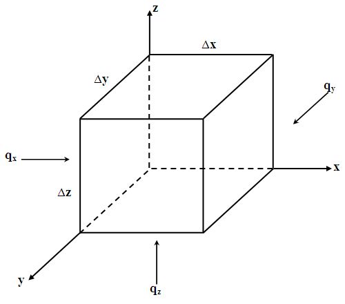
 Fig. 5.1. Control volume for flow through a confined aquifer.

 

As we know that the actual fluid motion can be subdivided on the basis of the components of flow parallel to the three principal axes (i.e., X, Y and Z). If q is flow per unit cross-sectional area, ρ_w q_x is the portion of mass flow (flux) parallel to the X-axis, and so on, where ρ_w is the fluid density (density of water in the present case).

 

The mass flux into the control volume is: ρ_w q_x  ∆y ∆z along the X-axis. The mass flux out of the control volume is: 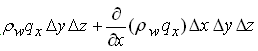. Since there are flow components along all the three axes, similar terms can be determined for the other two directions. The continuity equation is given as:

 

Mass inflow rate – Mass outflow rate = Change of mass storage with time  (5.1)

 

For the control volume, the term on the left hand side of Eqn. (5.1) represents net mass flux (inflow rate –outflow rate) into the control volume. Thus, the net mass flux of water in X-, Y- and Z-directions are given as:

 

Net flux in X-direction = 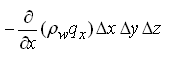     (5.2)

 

Net flux in Y-direction =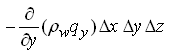  (5.3)

     

Net flux in Z-direction = 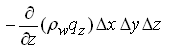     (5.4) 

   

 

Combining Eqns. (5.2), (5.3) and (5.4) yields the sum of water inflow rate minus the sum of water outflow rate for the control volume as:

 

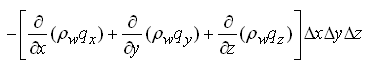             (5.5)

 

Now, the change in groundwater storage within the control volume is the change of water storage per unit time, which is expressed as:

 

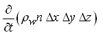                                                                  (5.6)

 

Where, n is the porosity of the aquifer.

 

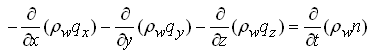
According to Eqn. (5.1), the net rate of water inflow is equal to the change in storage. Therefore, equating Eqns. (5.5) and (5.6) and dividing both sides by   ∆x ∆y ∆z gives:

 

            

 

After differentiating the term on the right hand side, the above equation can be rewritten as follows:

 

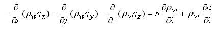            (5.7)

 

First term on the right hand side of Eqn. (5.7) denotes the mass rate of water produced by the expansion of water due to a change in density, which is controlled by the compressibility of water (β).  Second term on the right hand side of Eqn. (5.7) denotes the mass rate of water produced by the compaction of the porous medium (aquifer) as reflected by the change in porosity (n), which is controlled by the compressibility of the aquifer material (α).

 

We know that the change in ρ_w and change in n are both produced by a change in hydraulic head (h) and that the volume of water produced by the two mechanisms for a unit decline in head is called specific storage (S_s) which is expressed as, S_s = . As the mass rate of water produced (time rate of change of fluid mass storage) is , Eqn. (5.7) can be written as:

 

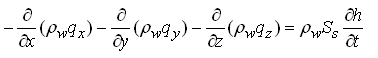                     (5.8)

 

Expanding the left hand side by chain rule and recognizing the fact that the terms of the form are  much greater than the terms of the form ,  allows us to neglect the second term, i.e. , . Then, Eqn. (5.8) becomes:

 

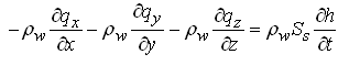                (5.9a)

 

 Since r_w is common on both sides of Eqn. (5.9a), it can be eliminated which reduces Eqn. (5.9a) to:

 

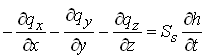                (5.9b)

 

 

From the Darcy’s law, we have:

 

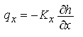                  (5.10)

 

                 (5.11)

 

                     (5.12)

 

Substituting Eqns. (5.10), (5.11) and (5.12) into Eqn. (5.9b) yields the main equation of groundwater flow:

 

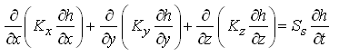                        (5.13)

 

Where, K_x, K_y and K_z = aquifer hydraulic conductivities in the X-, Y- and Z- directions, respectively; S_s = specific storage of the aquifer; h = hydraulic head in the aquifer; and t = time.

 

Equation (5.13) is a general equation for transient three-dimensional flow through a heterogeneous and anisotropic saturated porous medium.  In this equation, spatial coordinates x, y and z, and time t are independent variables and hydraulic head (h) is a dependent variable. The parameters of this equation are K_x, K_y, K_z and S_s. Note that Eqn. (5.13) is second order in x, y and z while first order in t. The physical meaning of the terms on the left hand side of Eqn. (5.13) is ‘net outflow rate of groundwater per unit volume of the aquifer’, whereas the term on the right hand side represents ‘time rate of change of groundwater volume within the unit volume of the aquifer’.

 

5.3 Equations for Groundwater Flow in Confined Aquifers

Since Eqn. (5.13) is a general equation of groundwater flow, it can be written in many forms that apply to a variety of different flow conditions. Some of these alternative equations are presented in subsequent sections for two extreme cases: (i) the most complex case, i.e., heterogeneous and anisotropic aquifer systems, and (ii) the simplest case, i.e., homogeneous and isotropic aquifer systems.

 

5.3.1 Heterogeneous and Anisotropic Confined Aquifer System

Although Eqn. (5.13) is called a general equation for groundwater flow, it essentially represents three-dimensional (3-D) transient flow through heterogeneous and anisotropic confined aquifers. 

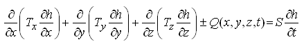
Multiplying both sides of Eqn. (5.13) by the aquifer thickness (b), we get another form of groundwater flow equation for heterogeneous and anisotropic confined aquifers:

                   

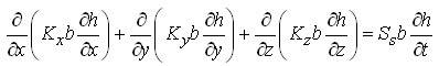
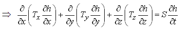              (5.14)

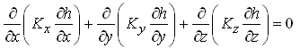
 Where, T_x, T_y and T_z are aquifer transmissivities in X-, Y- and Z-directions, respectively; S is the storage coefficient of the aquifer; and all other variables have the same meaning defined earlier. Moreover, under steady-state flow conditions in a heterogeneous and anisotropic confined aquifer system, there is no change in aquifer storage with time, i.e.=0, . Therefore, Eqn. (5.13) simplifies to: 

                  (5.15) 

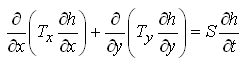
Moreover, for two-dimensional (2-D) transient groundwater flow in heterogeneous and anisotropic confined aquifer systems, Eqn. (5.13) can be written as: 

                               (5.16) 

and Eqn. (5.14) can be written as: 

                                             (5.17) 

5.3.2 Homogeneous and Isotropic Confined Aquifer System

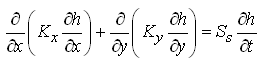
For homogeneous and isotropic confined aquifer systems, the hydraulic conductivity (K) will not vary with space and K_x = K_y = K_z = K. Therefore, Eqn. (5.13) simplifies to: 

                                 (5.18) 

Or, 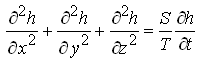                           (5.19)

 

Eqns. (5.18) and (5.19) represent transient groundwater flow through homogeneous and isotropic confined aquifer systems. As K/S_s or T/S is called ‘hydraulic diffusivity’ of the aquifer system, Eqns. (5.18) and (5.19) are known as three-dimensional (3-D) diffusion equations. 

For two-dimensional (2-D) groundwater flow through homogeneous and isotropic confined aquifer systems, Eqn. (5.18) simplifies to: 

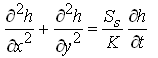                                           (5.20) 

and Eqn. (5.19) simplifies to: 

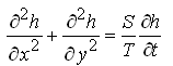                                     (5.21) 

Eqns. (5.20) and (5.21) are known as two-dimensional diffusion equations. 

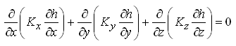
Under steady-state flow conditions in a homogenous and isotropic confined aquifer system, there is no change in storage with time, i.e., . Therefore, Eqns. (5.18) and (5.19) can be written as: 

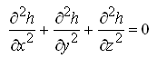                                         (5.22) 

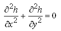
Eqn. (5.22) is known as the well-known three-dimensional Laplace equation. The two-dimensional Laplace equation is given as: 

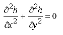                                         (5.23) 

Note that Eqns. (5.20), (5.21) and (5.23) as well as their one-dimensional forms are widely used for obtaining analytical solutions to specific field problems.

 

Furthermore, if a groundwater source or sink exists, Eqn. (5.13) is written as follows: 

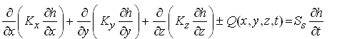           (5.24)

 

Where, Q is the volumetric source rate and/or sink rate per unit volume of the confined aquifer [L³T^-1/L³]. Note that if a groundwater source exists, there will be ‘+Q’ and if a groundwater sink exists, there will be ‘-Q’. Groundwater sources are recharge or inflow into the aquifer and groundwater sinks are pumping or outflow from the aquifer.

 

Equation (5.24) can be expressed in words as: 

Inflow rate – Outflow rate ± Source/Sink rate = Change of storage  (5.25) 

Multiplying both sides of Eqn. (5.24) by the aquifer thickness (b) yields: 

                (5.26) 

Under steady-state flow conditions, Eqn. (5.24) can be written as: 

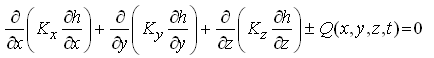        (5.27) 

5.4 Equations for Groundwater Flow in Unconfined Aquifers

As we know that the water from unconfined aquifers is released due to draining of water from pores (pore spaces). Unlike confined aquifers, the water released due the compressibility of aquifer material and water is generally negligible (i.e., S_s0). This drainage of pores results in a decline in the position of the water table, and hence the saturated thickness of unconfined aquifers changes with time. This is in contrast with the confined aquifer wherein although the hydraulic head (piezometric level) declines, the saturated thickness of the aquifer remains constant. Thus, the ability of unconfined aquifers to transmit water, i.e., aquifer transmissivity (T) changes with time. Such a hydraulic behavior of unconfined aquifers complicates the analysis of flow.

Since S_s0 in case of unconfined aquifers, the general equation of flow in unconfined aquifer systems is not represented by Eqn. (5.13). In principle, the location of the water table in space and time can be computed by solving the following equation: 

                 (5.28)

 

Note that the zero appears on the right hand side of Eqn. (5.28) because S_s is zero in case of unconfined aquifers, not because the flow is steady. To solve Eqn. (5.28) is a rigorous approach. Difficulty is that the water table position is the outcome of the solution yet the water table position is required (priori) to define the flow domain in which Eqn. (5.28) applies. This problem of unconfined aquifer flow was solved by Boussinesq in 1904 who analyzed the flow through unconfined aquifers using the Dupuit-Forchheimer (D-F) assumptions.

 

The Dupuit-Forchheimer (D-F) assumptions for an unconfined flow system are as follows (Fig. 5.2): 

(i)    Flow lines are assumed to be horizontal and equipotentials are vertical at any vertical cross section of the unconfined flow system.

(ii)     The hydraulic gradient is assumed to be equal to the slope of the free surface (water table) and to be invariant with depth.

  

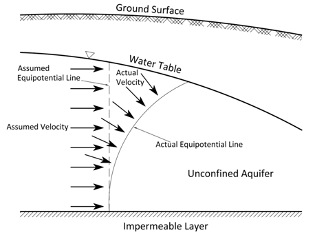
Fig. 5.2. Actual and assumed velocity distributions in unconfined aquifers.

 

5.4.1 Boussinesq Equation for Heterogeneous and Anisotropic Unconfined Aquifer System

Assume that the unconfined aquifer is heterogeneous and anisotropic. As the changes in density are unimportant in unconfined aquifers, mass balance is replaced by a volume balance for unconfined flow systems. For deriving groundwater flow equation for unconfined aquifers, let’s consider a small part of the unconfined aquifer (i.e., control volume) having three sides of lengths ∆x, ∆y and ∆h, respectively (Fig. 5.3); here h is the saturated thickness which varies with a decrease or increase in the water table position. Since the D-F assumptions neglect the vertical flow in unconfined aquifers, and therefore the actual fluid motion can be subdivided into q_x and q_y on the basis of the two components of flow parallel to the X-axis and Y-axis, respectively where q denotes the flow per unit cross-sectional area of the aquifer.   

 

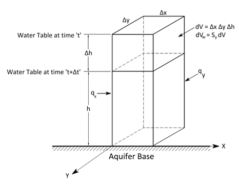
Fig. 5.3. Control volume for flow through an unconfined aquifer.

 

The net volumes of flow in X- and Y-directions are given as: 

Net volume of flow in X-direction = 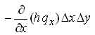                              (5.29) 

Net volume of flow in Y-direction = 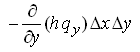                            (5.30)

 

The rate of change in groundwater storage within the control volume is given as . Now, from the continuity principle, net outflow rate is equal to the rate of change in groundwater storage within the control volume. That is,

 

                     (5.31)

From the Darcy’s law 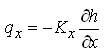,  and 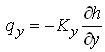, and also ∆x ∆y is common on both sides which allows us to eliminate it. Thus, Eqn. (5.31) can be written as: 

                          (5.32)

 

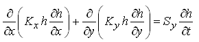
Where, K_x and K_y = aquifer hydraulic conductivities in the X- and Y-directions, respectively; S_y = specific yield of the aquifer; h = hydraulic head in the aquifer; and t = time.

 

Equation (5.32) is known as ‘nonlinear Boussinesq equation’ or simply ‘Boussinesq equation’, which is a general equation for transient two-dimensional flow in heterogeneous and anisotropic unconfined aquifer systems. This equation is a type of differential equation that cannot be solved using calculus, except for some very specific cases.   

If the drawdown in an unconfined aquifer is very small compared to its saturated thickness, the variable aquifer thickness (h) can be replaced with an average saturated thickness of the unconfined aquifer (h_mean) which is assumed to be constant over the aquifer. Given this assumption, the Boussinesq equation [Eqn. (5.32)] can be linearized as follows: 

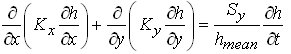                                                   (5.33)

 

Equation (5.33) is known as ‘linear Boussinesq equation’, which can easily be solved using calculus. For steady-state groundwater flow in heterogeneous and anisotropic unconfined aquifer systems ,  (i.e., no change in aquifer storage with time). Therefore, Eqn. (5.32) simplifies to: 

                        (5.34) 

and Eqn. (5.33) simplifies to: 

                            (5.35)

Moreover, if a groundwater source or sink exists, Eqn. (5.32) is written as: 

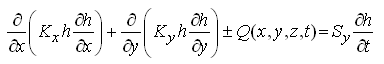                  (5.36) 

For steady-state groundwater flow conditions, Eqn. (5.36) can be written as: 

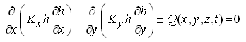                         (5.37)

 

5.4.2 Boussinesq Equation for Homogenous and Isotropic Unconfined Aquifer System

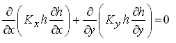
For homogeneous and isotropic unconfined aquifer systems, K_x = K_y = K and the value of K will remain constant over the aquifer. Therefore, for groundwater flow through homogeneous and isotropic unconfined aquifer systems, Eqn. (5.32) reduces to: 

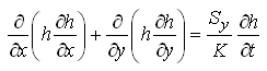                          (5.38) 

Note that Eqn. (5.38) is also called ‘nonlinear Boussinesq equation’, and it cannot be solved using calculus, except for some simple cases. 

For homogeneous and isotropic unconfined aquifer systems, Eqn. (5.33) simplifies to: 

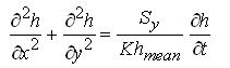                                 (5.39a) 

Or, 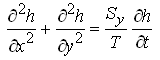                                      (5.39b)

 

Equations (5.39a) or (5.39b) is called ‘linear Boussinesq equation’, which are widely used for obtaining analytical solutions, together with their one-dimensional forms. Note that Eqn. (5.39a) or Eqn. (5.39b) has the same form as that for homogeneous and isotropic confined aquifer systems [i.e., Eqn. (5.19)]. 

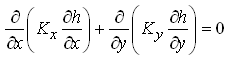
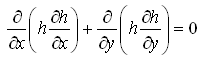
For steady-state groundwater flow conditions in homogeneous and isotropic unconfined aquifer systems, Eqn. (5.34) can be written as: 

                                  (5.40)

and Eqn. (5.35) can be written as: 

                                         (5.41)

 

Equation (5.41) is the same as Eqn. (5.23), i.e., ‘two-dimensional Laplace equation’. 

5.5 Equations for Groundwater Flow in Leaky Confined Aquifers

The equations of confined aquifers presented in Sections 5.2 and 5.3 are based on the assumption that all flow comes from water stored in the aquifer. However, in reality, significant flow is often generated from leakage into the confined aquifer through overlying or underlying confining layers (Fig. 5.4). If this is the case, then the confined aquifer is called ‘leaky confined aquifer’. The procedures for the derivation of governing equation for flow in leaky confined aquifers are the same as discussed in Section 5.2, except for an additional term ‘leakage’ and the two-dimensional flow in case of leaky confined aquifers. 

 

The leakage is considered to appear in the control volume (Fig. 5.1) as horizontal flow. This assumption is justified on the grounds that the hydraulic conductivity of the aquifer is usually much greater than that of the confining layer (aquitard). For these conditions, the law of refraction suggests that the flow in the confining layer will be almost vertical if the flow in the confined aquifer is horizontal as illustrated in Fig. 5.4. Thus, the flow in leaky confined aquifers is essentially two-dimensional in the horizontal plane. Given these flow conditions in leaky confined aquifers, the general equation of flow can be derived using the law of mass conservation and Darcy’s law as presented below.

  

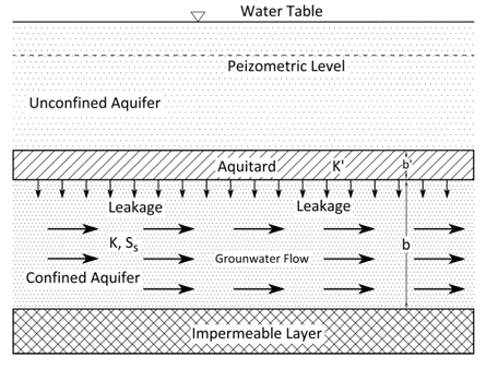
Fig. 5.4. Groundwater flow pattern in a leaky confined aquifer.

 

5.5.1 Heterogeneous and Anisotropic Leaky Confined Aquifer System

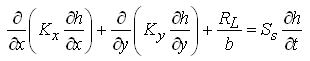
Let’s assume a heterogeneous and anisotropic leaky confined aquifer of thickness b, which receives leakage (R_L) from an overlying unconfined aquifer (Fig. 5.4). Considering the above-mentioned flow conditions in leaky confined aquifers, the mass balance of flow for a control volume (Fig. 5.1) yields the following equation: 

        (5.42) 

Dividing both sides of Eqn. (5.42) by ∆x∆y, we have: 

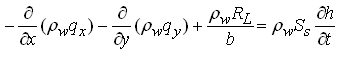                         (5.43) 

By assuming that the density of water does not vary spatially, i.e., ρ_w = constant over the aquifer, the density term can be taken out and thereby ρ_w gets eliminated. Thus, Eqn. (5.43) reduces to:

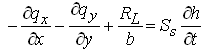                                  (5.44)

 

From the Darcy’s law 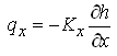,  and  . Substituting these expressions of q_x and q_y into Eqn. (5.44) yields the general equation of flow for heterogeneous and anisotropic leaky confined aquifers: 

                       (5.45)

 

Multiplying both sides of Eqn. (5.45) by b (thickness of the leaky confined aquifer), we get another form of general groundwater flow equation for heterogeneous and anisotropic leaky confined aquifers:

 

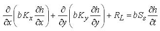
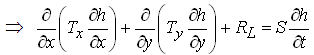                            (5.46)

 

Where, K_x and K_y= hydraulic conductivities of the leaky confined aquifer in X- and Y- directions, respectively; R_L = leakage into the leaky confined aquifer; h = hydraulic head in the leaky confined aquifer; S_s = specific storage of the leaky confined aquifer; S = storage coefficient of the leaky confined aquifer; and T_x and T_y = transmissivities of the leaky confined aquifer in X- and Y- directions, respectively.

 

The leakage rate (R_L) can be computed from the Darcy’s law as follows:

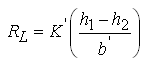                                              (5.47)

 

Where, h₁ = hydraulic head at the top of the aquitard (leaky confining layer), h₂ = hydraulic head in the aquifer just below the aquitard, = vertical hydraulic conductivity of the aquitard, and = thickness of the aquitard. 

Note that if an additional source of recharge and/or a sink (e.g., pumping) occurs in case of leaky confined aquifer systems, they should also be included in Eqns. (5.45) and (5.46) along with the leakage (R_L). 

5.5.2 Homogeneous and Isotropic Leaky Confined Aquifer System

For homogeneous and isotropic leaky confined aquifer systems, K_x = K_y = K and the value of K will remain constant over the aquifer. Therefore, for groundwater flow through homogeneous and isotropic leaky confined aquifer systems, Eqn. (5.45) can be written as: 

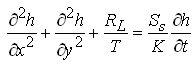                                   (5.48)

and Eqn. (5.46) can be written as: 

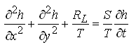                                     (5.49)

 

5.6 Solution of Groundwater Flow Equations

Flow of water in aquifer systems (saturated porous media) can be mathematically described by the above equations according to the flow conditions under investigation. They all are partial differential equations in which the hydraulic head (h) is a dependent variable. They are solved by using a mathematical model consisting of the applicable governing flow equation, boundary conditions, and initial conditions. If the aquifer is homogenous and isotropic, and the boundaries can be described with algebraic equations, then the mathematical model can be solved by an analytical technique based on integral calculus.

 

However, for heterogeneous and anisotropic aquifer systems (e.g., layered aquifer systems), a numerical solution to the mathematical model is required. Numerical solutions are based on the concept that the partial differential equation can be replaced by a similar equation that can be solved using arithmetic. Similarly, the equations governing boundary and initial conditions are replaced by numerical statements of these conditions. Numerical solutions are obtained using well-known numerical techniques such as ‘Finite Difference Method’ (FDM), ‘Finite Element Method’ (FEM), ‘Method of Characteristics’ (MOC), ‘Collocation Method’ (CM), and Boundary Element Method (BEM), of which FDM and FEM are widely used by groundwater hydrologists or hydrogeologists. Numerical solutions are generally solved on computers, and the entire modeling process is known as ‘numerical modeling’. Fundamentals of groundwater modeling are discussed in Chapter 22.   

 

References

Freeze, R.A. and Cherry, J.A. (1979). Groundwater. Prentice Hall, NJ.

Todd, D.K. (1980). Groundwater Hydrology. John Wiley & Sons, New York.

 

Suggested Readings

Bear, J. (1979). Hydraulics of Groundwater. McGraw-Hill, New York

Freeze, R.A. and Cherry, J.A. (1979). Groundwater. Prentice Hall, NJ.

Fetter, C.W. (2000). Applied Hydrogeology. Fourth Edition. Prentice Hall, NJ.

Sarma, P.B.S. (2009). Groundwater Development and Management. Allied Publishers Pvt. Ltd., New Delhi.