Ground Water, Wells and Pumps

Lesson 6 Analysis of Steady Groundwater Flow

6.1 Steady Flow in Confined Aquifers

If there is a steady movement of groundwater in a confined aquifer, there will be a linear gradient or slope to the piezometric surface; i.e., its two-directional projection is a straight line. For this type of groundwater flow, Darcy’s law can be directly applied. In Fig. 6.1, a portion of a homogeneous and isotropic confined aquifer of uniform thickness is shown wherein the hydraulic head has a linear gradient. Two observation wells/piezometers are installed L distance apart in the aquifer where the hydraulic head can be measured. 

Using Darcy’s law, the quantity of groundwater flow per unit width of the aquifer (q) can be determined as: 

                                                            (6.1)

Where, K = mean hydraulic conductivity of the confined aquifer, b = thickness of the confined aquifer, and = hydraulic gradient in the X-direction.

 

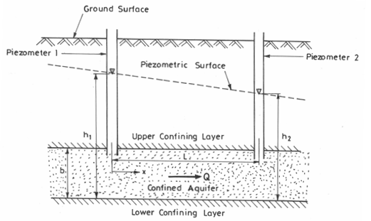
Fig. 6.1. Steady flow through a confined aquifer of uniform thickness.          (Modified from Fetter, 1994)

 

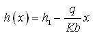
One may be interested to know the hydraulic head (h) at some intermediate distance, x between Piezometer 1 having hydraulic head h₁ and Piezometer 2 having hydraulic head h₂. This can be determined from the following equation: 

                                                 (6.2)

 

Where, h(x) = hydraulic head at distance x, and x = distance from Piezometer 1.

 

6.2 Steady Flow in Unconfined Aquifers

In unconfined aquifers, as illustrated in Fig. 6.2, the fact that the water table constitutes the upper boundary of the groundwater flow region complicates flow determination. The shape of the water table determines the flow distribution, but at the same time the flow distribution governs the water-table shape. Therefore, a direct analytical solution of the Laplace equation is not possible in this case. 

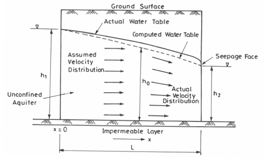
Fig. 6.2. Steady flow in an unconfined aquifer between two water bodies with vertical boundaries. (Modified from Todd, 1980) 

Moreover, the saturated thickness of unconfined aquifers decreases in the direction of flow (Fig. 6.2).  If there is no recharge or evaporation, the quantity of water flowing through the left side (upstream end) is equal to that flowing through the right side (downstream end). From Darcy’s law, it is obvious that since the cross-sectional area is smaller on the right side, the hydraulic gradient must be greater on this side. Thus, the water-table gradient in unconfined flow is not constant; rather it increases in the direction of flow.

The above problem was solved by Dupuit in 1863 by adopting certain simplifying assumptions, which are well-known as the Dupuit assumptions or Dupuit-Forchheimer assumptions. These assumptions are: (i) the hydraulic gradient in an unconfined flow system is equal to the slope of the water table, and (ii) for small water-table gradients, the streamlines are horizontal and the equipotential lines are vertical. Solutions based on these assumptions have proved to be very useful in many practical problems. However, the Dupuit assumptions do not allow for a seepage face above the outflow side (Fig. 6.2). Furthermore, since the slope of the parabolic water table increases in the direction of flow, the Dupuit assumptions become increasingly poor approximations to the actual flow; therefore, the actual water table deviates more and more from the computed water table in the direction of flow (Fig. 6.2). Thus, the actual water table always lies above the computed water table. The reason for this can be explained by the fact that the Dupuit flows are assumed to be horizontal, whereas the actual velocities of the same magnitude have a downward vertical component so that a greater saturated thickness (i.e., larger height of the water table from the aquifer base) is required for the same discharge.

 

6.2.1 Steady Unconfined Flow without Recharge or Evapotranspiration

For steady unconfined flow without recharge or evapotranspiration, given the Dupuit assumptions, Darcy’s law can be applied to determine groundwater discharge per unit width of the aquifer (q) at any vertical section: 

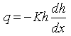                                                          (6.3)

 

Where, h = saturated thickness of the unconfined aquifer, K = mean hydraulic conductivity of the unconfined aquifer, and = hydraulic gradient in the X-direction. 

Applying boundary conditions, i.e., at x = 0, h = h₁; at x = L, h = h₂ (Fig. 6.2), Eqn. (6.3) can be integrated with these boundary conditions as:

 

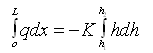
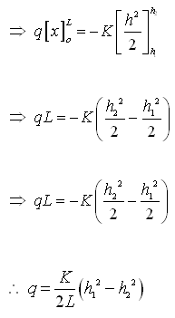           (6.4)

 

Where, L = flow length, h₁ = head at the origin (at x = 0), and h₂ = head at a distance L (at x = L).

 

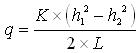
Equation (6.4) is known as the Dupuit equation, which indicates that the water table is parabolic in form. For flow between two fixed water bodies of constant heads h₁ and h₂ as shown in Fig. 6.2, the water-table slope at the upstream boundary of the aquifer (neglecting the capillary zone) can be given as: 

                                                  (6.5) 

However, the boundary h = h₁ is an equipotential line because of the constant fluid potential in the water body. Consequently, the water table must be horizontal at this section, which is inconsistent with Eqn. (6.5).

 

It should be noted that because of the Dupuit-Forchheimer assumptions, many discrepancies arise. Nevertheless, for flat water-table slopes, where the sine and tangent are nearly equal, the Dupuit equation [Eqn. (6.4)] closely predicts the water-table position except near the downstream portion. In general, the Dupuit equation accurately determines q or K for the given boundary heads. 

6.2.2 Steady Unconfined Flow with Recharge or Evapotranspiration

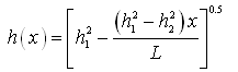
For steady one-dimensional unconfined flow subject to recharge or evapotranspiration, as shown in Fig. 6.3, we can obtain the following equation for the water-table position: 

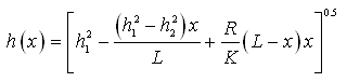                                                        (6.6) 

Where, h (x) = hydraulic head (water-table height from the aquifer base) at a distance x from the origin (upstream end), x = distance from the origin, L = distance from the origin to the point where h₂ is measured, h₁ = head at the origin (upstream end), h₂ = head at the distance L (downstream end), K = mean hydraulic conductivity of the unconfined aquifer, and R = recharge rate.

 

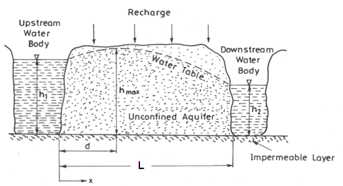
Fig. 6.3. Steady unconfined flow subject to recharge.

(Modified from Fetter, 1994)

Equation (6.6) can be used to find the height of the water table (from the aquifer base) anywhere between two points located L distance apart if the saturated thickness of the unconfined aquifer is known at the two end points (i.e., h₁ and h₂ are known). It should be noted that if significant evapotranspiration (ET) occurs instead of recharge (R), then in Eqn. (6.6), the term R will be replaced by ET with negative sign (i.e., - ET) . 

In the absence of recharge or evapotranspiration, Eqn. (6.6) will reduce to: 

                                           (6.7)

 

Equation (6.7) is called Dupuit parabola.

 Now, by differentiating Eqn. (6.6) and considering q_X= , it can be shown that the discharge per unit width at any section x distance from the origin   is given by: 

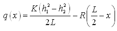                                                                                   (6.8) 

If the water table is subject to recharge (R), there may be water divide with a crest in the water table (known as ‘groundwater divide’). In this case, q(x) will be zero at the groundwater divide. If d is the distance from origin to groundwater divide, then substituting q(x) = 0 and x = d into Eqn. (6.8) yields: 

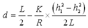                                                  (6.9) 

Where, all the variables have the same meaning as defined earlier. 

If the distance from the origin to the groundwater divide has been found, then the water-table height (from the aquifer base) at the groundwater divide (i.e., h_max) can be determined by replacing x with d in Eqn. (6.6). That is, 

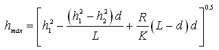                         (6.10) 

In Eqn. (6.10), all the variables have the same meaning as defined earlier.

 

 

6.3 Example Problems

6.3.1 Problem 1

A confined aquifer is 3.0 m thick. The piezometric level drops 0.15 m between two observation wells which are located 238 m apart. The hydraulic conductivity of the aquifer is 6.5 m/day and the effective porosity is 0.15. Determine the following: (a) Discharge of groundwater through a strip of the aquifer having 10 m width, and (b) Average linear velocity of groundwater.

 

Solution: From the question, we have:

Thickness of aquifer, b = 3.0 m

Difference in piezometric levels, Δh = 0.15 m

Distance between the observation wells, ΔL = 238 m

Hydraulic conductivity of the aquifer, K = 6.5 m/day

Effective porosity, n_e = 0.15

Width of the aquifer strip, W = 10 m

 

(a) Groundwater discharge per unit width of the confined aquifer (q) is given as:

                            

                                            

 

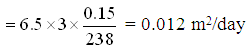
Groundwater discharge through the 10 m aquifer strip = W × q = 10 × 0.012

= 0.12 m³/day, Ans.

 

(b) Average linear velocity of groundwater =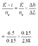 

                                                                 = 0.027 m/day, Ans.

 

6.3.2 Problem 2

An unconfined aquifer has a hydraulic conductivity of 1.2×10^-2 cm/s. There are two fully penetrating observation wells installed in this aquifer, which are separated by a distance of 98.5 m from each other. In the upstream observation well, the water level is 7.5 m above the aquifer bottom, and in the downstream observation well, it is 6.0 m above the aquifer bottom.

(i) What is the groundwater discharge per 40 m-wide strip of the aquifer? Express your answer in cubic meters per day.

(ii) What is the water-table elevation at a point midway between the two observation wells?

 

Solution: From the question, we have:

Hydraulic conductivity of the aquifer, (K) = 1.2 × 10^-2 cm/s = 1.2 × 10^-4 m/s

Distance between the two observation wells, L = 98.5 m.

Considering bottom of the aquifer as a datum, hydraulic head at the upstream observation well (h₁) = 7.5 m, and hydraulic head at the downstream observation well (h₂) = 6.0 m.

Width of the aquifer strip, W = 40 m

 

(i) Groundwater discharge per unit width of the unconfined aquifer (q) is given as:

 

 

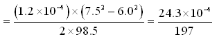
   = 1.23 × 10^-5 m²/s

 

Groundwater discharge per 40 m-wide aquifer strip = W × q

                                                                          = 40 × (1.23 × 10^-5)

                                                                          = 49.2 × 10^-5 m³/s

                                                                          = 42.51 m³/day, Ans.

 

(ii) Distance of the point midway between the two observation wells (x) = 98.5/2 = 49.25 m. Water-table elevation at the point midway between two observation wells (h_mid) can be calculated from the following equation: 

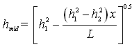                             , where x = 49.25 m 

                         

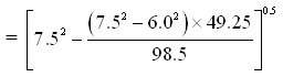
                          Ans.

References

Fetter, C.W. (1994). Applied Hydrogeology. Third Edition, Prentice Hall, NJ.

Todd, D.K. (1980). Groundwater Hydrology. John Wiley and Sons, New York.

 

Suggested Readings

Sarma, P.B.S. (2009). Groundwater Development and Management. Allied Publishers Pvt. Ltd., New Delhi.

Fetter, C.W. (2000). Applied Hydrogeology. Fourth Edition, Prentice Hall, NJ.

Todd, D.K. (1980). Groundwater Hydrology. John Wiley and Sons, New York.