Irrigation Engineering

LESSON 45 Evaluation of Drip Emitters and Design of Drip Irrigation System

45.1 Performance Evaluation Drip Emitters

The different characteristics used for performance evaluation of emitters are as follows:

a)     Manufacturing Characteristics

b)    Hydraulic Characteristics

c)     Operational Characteristics

 

a) Manufacturing Characteristics

The variations in passage size, shape, surface and finish that occur are small in absolute magnitude but represent a relatively large percent variation. Although pressure compensating emitters use an elastomeric material to achieve consistent dimensions and characteristics. The amount of difference to be expected varies with the design of the emitter materials used in its construction and the care with which it is manufactured. The emitter coefficient of manufacturing variation (v) is used as a measure of the anticipated variations in discharge in a simple of new emitters. The value of C_v should be available from the manufacturer or it can be estimated from the measured discharges of a sample set of at least 50 emitters operated at a reference pressure head. It is estimated as

 C_v  = Standard Deviation (s) / Average Flow rate (q)

 

The system coefficient of manufacturing variation (v_s) is a useful concept because more than one emitter or emission points may be used per plant. In such a situation the variations in flow rate for each emitter around the plant partly compensate for one another.

 The value of v_s can be computed by following equation (US Soil Cons. Service, 1984):

                                                                                                              (45.1)

In which

V= emitter coefficient of manufacturing variation.

e^' minimum number of emitters per plant or 1 if one emitter is shared by more than one plant.

 

Table 45.1 provides interpretation of drip emitters based on manufacturing coefficient of variation.

 

Table 45.1. ASAE Interpretation on Manufacturing Coefficient of Variation

Emitter type	Cv	Interpretation
Point Source	< 0.05 0.05 - 0.07 0.07 - 0.11 0.11- 0.15       > 0.15	Excellent Average Marginal Poor Unacceptable
Line Source	< 0.10 0.10 - 0.20        > 0.20	Good Average Marginal to    Unacceptable

 

b) Hydraulic Characteristics

The relationship between changes in pressure head and discharge is an important characteristic of emitters. The pressure compensating emitters have a low value of the exponent. However since they have some physical part that responds to pressure their long range performance requires careful consideration. The compensating emitters usually have a high coefficient of manufacturing variation (v), and their performance may be affected by temperature, material fatigue or both. On undulating terrain the design of a highly uniform system is usually constrained by the pressure sensitivity of the average emitter. Compensating emitters provide the solution. Emitters of various sizes may be placed along the lateral to meet pressure variations resulting from changes in elevation. In laminar flow emitters which include the long path, low discharge devices the relation between the discharge and the operating pressure is linear, i.e., doubling the pressure doubles the discharge. Therefore the variations in operating pressure head within the system are often kept to within ± 5 percent of the desired average. In a turbulent flow emitter the change in discharge varies with the square root of the pressure head, i.e., x = 0.5, and the pressure is to be increased four times to double the flow. Therefore the pressure head in drip irrigation system with turbulent flow emitter is often allowed to vary by ± 10% of the desired average (US Soil Cons. Service, 1984).

 Depending upon the experimental values of x, flow regimes can be obtained. Based on the flow regime and exponent x the emitters can be classified (Table 45.2).

 

Table 45.2. Emission device classification

Flow Regime	x - Value	Emitter Type
Variable flow path	0.0 0.1 0.2 0.3	Pressure compensating
Vortex flow	0.4	Vortex
Fully turbulent flow	0.5	Orifice tortuous
Mostly turbulent flow	0.6 0.7 0.8	Long or spiral path
Mostly laminar flow	0.9	Micro tube
Fully laminar flow	1.0	Capillary

 

c) Operational Characteristics

The coefficient of uniformity proposed by Christiansen (1948) is widely accepted for estimating uniformity of water application through sprinkler irrigation systems. However this measure determines the uniformity of sprinkling pattern of one nozzles of sprinkler irrigation system. This is not required for the emitter of drip irrigation system. Hence the Christiansen formula is not used in drip systems are significantly different from those of sprinkler nozzles. The uniformity in water application of emitters (expect of pressure compensating type emitters) is influenced by the operating pressure, emitter spacing, land slope, size of the pipe line, emitter discharge, and emitter discharge variability of specified emitters. The emitter discharge variability is due to the variation in operating pressure and temperature, manufacturing variability (coefficient of variation, C_v), clogging, and aging of the emitters.

Karmeli and Keller (1975) proposed the ‘emission uniformiy’ as the measure for the performance evaluation of the drip irrigation system. They proposed two measures viz. emission uniformity and absolute emission uniformity. These measures are now widely accepted to measure the performance of irrigation system when laid in the field.

Emission Uniformity (EU): The Primary objective of the good drip irrigation system is to provide sufficient water or discharge to adequately irrigate the least watered plant or area. Therefore the relation between the minimum and average emitter discharge within the subunit of the system is most important factor and is designated by the emission uniformity.

The emitter discharge from minimum four emitters (in case of more than one emitters per plant, the discharges are taken from all the emitters at minimum four locations or plants and the discharges from each location are averaged) per lateral along four randomly selected laterals are measured. The minimum 16 measurement points so selected should include the extremes and uniformly spaced in the subunit. This can be achieved by selecting the first, one third point, two third point and the last emitter on a selected lateral.

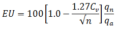
The emission uniformity, EU, which is expressed as percentage is the ratio of the average emitter discharge from the lowest one fourth of the field data (obtained from arranging the emitter discharges in descending order) to the average discharge of all the data.EU is computed by:

 EU =  × 100

 Where,

q_n = average of the lowest one fourth of the field data emitter discharges (Lh^-1),

q_a = average of all the field data emitted discharges (Lh^-1),

Absolute emission Uniformity: Corp quality and productivity may be affected by both excess watering and under watering. Therefore the uniformity measure needs to include the maximum and minimum emitter discharges and the uniformity. The measurements that need to undertake in the field is same as for the computation of the computation of the emission uniformity. The absolute emission uniformity is computed by the following formula.

 EU_a  =

 

where,

q_x = average of the highest one – eighth of the field data emitter discharges, (Lh^-1)

 The emission uniformity measures proposed above are used to measure the field performance of the already installed drip irrigation system and therefore these are also called as field emission uniformity and absolute field emission uniformity, respectively,

 However the emission uniformity measures are also required at the time of design and need to be estimated before installing the system in the field. These are called as design emission uniformity and absolute design emission uniformity, respectively. In this case, the measurements for qa, qn and qx are not available, These are estimated form the pressure – discharge relationship of the emitter. For example, qn is the minimum emitter discharge computed with the minimum pressure using the pressure using the pressure discharge relationship. In this way qa and qx are estimated. The corresponding formulas are:

 Emission Uniformity (EUd)

               (45.2)

In which,

EU = design emission uniformity, %

n = (i) for point source emitter on a perennial tree crop, number of emitters per plant, (ii) for a line source emitters on a perennial tree crop, either the rooting diameter of the plants divided by the same unit length of lateral used to compute C_V or 1, whichever is greater.

C_v = the manufacture’s coefficient of variation for point source or line source emitters,

q_n = the minimum emitter discharge at a minimum pressure in the section (sub unit), computed from pressure discharge relationship,Lh^-1.

q_a = the average or design emitter discharge for the section (sub- unit), Lh^-1.

 

The commonly recommended ranges for the design emission uniformity are as follows:

i) Point source emitters for tree crops with spacing larger than 4 m:

a) Land slope less than 2% - (E_u 90 to 95%)                                     

b) Land slope greater than 2% -( E_u 85 to 90%)

 

ii) Point source emitters for tree crops with spacing larger than 4 m:

a) Land slope less than 2% -    (E_u 85 to 90% )

b) Land slope greater than 2% - (E_u 80 to 90%)

 

iii) Line source emitters on annual or perennial crops:

a) Land slope less than 2% -   (E_u 80% to 90%)

b) Land slope greater than 2% -   (E_u 75 to 85%)

 

45.2 Evaluation of Emission Uniformity

Example 45.1: Determine the emission uniformity of a drip system section that uses drip emitter with coefficient of discharge (k_d) = 0.3, exponent (x) = 0.57 and coefficient of variation (C_v) = 0.06. Two emitters are used for each plant. The average pressure is 120 kP_a and minimum pressure is 90 kP_a.

 Solution:   

                        

                            = 0.3 × (90)^0.57

                           = 0.3 × 12.99

                           = 3.89 Lh^-1

               

                           = 0.3 × 15.31          

                           = 4.59 Lh^-1  

                    

                          = 100

                          = 80.1 %

The value of EU in Example 45.1 is lower than the recommended value stated above. The EU could be improved by reducing the difference between q_min and q_a (by using the emitters with lower values of the discharge exponent) or by using an emitter with a lower C_v.

 

45.3 Design of Drip Irrigation System

Example 45.2: Design a drip irrigation system for a citrus orchard of 1 ha area with length and breadth of 100 m each. Citrus has been planted at a spacing of 5 m ´ 5.5 m. The maximum pan evaporation during summer is 8 mm/day. The other relevant data are given below:

Land slope = 0.40 % upward slope from S – N direction,

Water source = A well located at the S–W corner of the field

Soil texture           = Sandy loam, Clay content = 18.4 %, Silt = 22.6 %,Sand     =59.0%, Field capacity = 14.9 %, Wilting point = 8 %,Bulk density = 1.44 g/cc,

Effective root zone depth = 120 cm, Wetting Percentage   = 40 %,

Pan coefficient = 0.7,Crop coefficient = 0.8

 

Solution:

Solution of this Example is taken from Tiwari (2009).

 

Step 1:

Estimation of Water Requirement

Evapotranspiration of the crop = Open pan evaporation X´ Pan coefficient X´ Crop  coefficient

                                               = 8 X 0.7 X 0.8

                                               = 4.48 mm/day

 

Volume of water to be applied = Area covered by each plant X Wetting fraction X Evapotranspiration of the crop

                                               = (5 X 5.5) X 0.40 X 4.48

                                               = 49.28 L day^-1 or 50 L day^-1

 

Step 2:

Emitter Selection and Irrigation Time

Emitters are selected based on the soil texture and crop root zone system. Assuming three emitters of 4 L h^-1, placed on each plant in a triangular pattern are sufficient so as to wet the effective root zone of the crop.

Total discharge delivered in one hour = 4 ´ 3 = 12 L h^-1

Irrigation time = 50 / 12 = 4 h 10 minutes

 

Step 3:

Discharge through Each Lateral 

A well is located at one corner of the field. Sub mains will be laid from the centre of field (Fig. 45.1). Therefore, the length of main, sub mains, and lateral will be 50 m, 97.25 m, 47.5 m each respectively. The laterals will extend on both sides of the sub mains. Each lateral will supply water to 10 citrus plants.

 Total number of laterals   = (100/5.5) ´ 2 = 36.36 (Considering only 36)

Discharge carried by each lateral, Q_lateral = 10 ´ 3 ´ 4 = 120 L h^-1

Total discharge carried by 36 laterals = 120 ´ 36 = 4320 L h^-1

Each plant is provided with three emitters, therefore total number of emitters will be 36 ´ 10 ´ 3 =1080

Step 4:

Determination of Number of Manifolds

Assuming the pump discharge = 2.5 L s^-1 = 9000 L h^-1

Number of laterals that can be operated by each manifold = 9000/120 = 75

So only one manifold or sub mains can supply water to all the laterals at a time.

Step 5:

Size of Lateral

Once the discharge carried by each lateral is known, then size of the lateral can be determined by using the Hazen- Williams equation .(Equation 44.4)

The reduction factor (F) can be estimated as

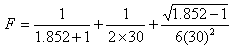
                                            = 0.367

                            

                              

                                 For D = 16 mm, = 0.063 m

 

The permissible head loss due to friction is 10% of head of 10 m (head required to operate 4 L h^-1 emitters) is 1 m, therefore 12 mm diameter. lateral size is selected.

Step 6:

Size of Sub Main

Total discharge through the sub mains =  Q_lateral X Number of laterals

                                                          = 120 X 36

                                                          = 4320 L h^-1 = 1.2 L s^-1

Assuming the diameter of the sub mains as 50 mm. The values of parameter of the Hazen- Williams equation are

       = 150

        = 1.2 L s^-1

       = 50 mm

        = 1.22 ´ 10¹²

         = 0.364

 

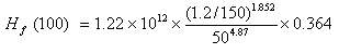
              = 0.31 m

H_f for 97.25 m of pipe length   = 0.31  ´ (97.25/100)

                                                 = 0.30 m

Therefore, frictional head loss in the sub mains = 0.30 m

Head at the inlet of the sub mains = H _emitter + H_{f lateral} + H_{f sub main} + H _slope

                                                    = 10 + 0.26 + 0.30 + 0.40

                                                    = 10.96 m

 

Pressure head variation =

                                      = 6.38 %

 

Estimated head loss due to friction in the sub main is much less than the recommended 20% variation, hence reducing the pipe size from 50 to 35 mm will probably be a good option.

 

                         

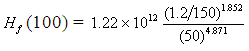
                                                     = 1.75 m

 

H_f for 97.25 m pipe = 1.75  ´ (97.25/100)

                                           = 1.70 m

Head at the inlet of the sub main = H _emitter + H_{f lateral} + H_{f sub main} + H _slope

                                                  = 10 + 0.26 + 1.70 + 0.40

                                                  = 12.36 m

Pressure head variation =

                                      = 17%

 

Pressure head variation lies within the acceptable limit, hence accepted.

Step 7:

Size of the main line

Assuming the diameter of main as 50 mm

Discharge of main, Q _main = Discharge of sub main,  Q_{sub main}

 

The values of parameter of the Hazen- Williams equation are

C = 150

  Q         = 1.2 L s^-1

    D     = 50 mm

  K       = 1.22 ´ 10¹²

 

              = 0.84 m

 

 for 50 m main pipe = 0.84 ´ (50/100)  = 0.42 m

 

Step 8.

Determining the Horse Power of Pump

Assume head variation due to uneven field variations and the losses due to pump fittings, etc. as 10 % of all other losses.

 

H_local  = 10 % of all other loss

Total dynamic head = ( H _emitter + H_{f lateral} + H_{f sub main} + H_{f main}+ H _slope )+H_static+H _local

                                 = 12.36 + 0.42 +10 +1.28

                                 = 29.06 m

 Pump Horse power                       

where,

 H = Total dynamic head, m

 Q = Total discharge through main line, L s^-1

η_p= Efficiency of pump                                             

 = 0.64   @ 1.0

 

Hence 1 hp pump or the pump giving 1.2L s^-1 discharge at head of 30.0 m is adequate for operating the drip irrigation system to irrigate for 1 ha area of citrus crop.

 

The design details of components micro irrigation system are estimated as

Length of laterals = 47.5 m,    Number of laterals         = 36,

Diameter of lateral = 12 mm, Length of sub main = 97.25 m,

Number of sub main = 1,        Diameter of sub main = 35 mm,

Length of main       = 50 m,     Number of main = 1,

Diameter of main   = 50 mm,  Total power required = 1 hp,

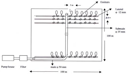
Fig. 45.1. Layout of designed drip irrigation system.

 

References

Bucks, D.A., Nakyama, P.S. and Warrick , A.W. (1982). Principles, Practices and Potentalines of Trickle (Drip) Irrigation, In Advances in Irrigation, Vol. 1, ed. Hillel, D. Academic Press, New York: 219-297.

Bureau of Indian Standards. (1984). Indian Standard IS 10799: 1984, Code of Practices of Design and Installation of Trickle Irrigation, Pub. Bureau of Indian Standards, Manak Bhawan, New Delhi.

Bureau of Indian Standards. (1999). Indian Standard IS 10799: 1999, Irrigation Equipment – Design, Installation and Field Evaluation of Micro- Irrigation Systems, Code of Practice, Pub. Burreau of Indian Standards, Manak Bhawan, New Delhi: 9.

Christiansen, JE. (1948). Irrigation by by Sprinkling California Agriculture Expt-Stat- Bullelin: 670.

Karmeli, D. and Keller, J. (1975). Trickle Irrigation Design, Rain Bird Sprinkler Manufacturing Corporation, Glendora, California, USA.

Schwab, G.O. Fangmeier, D.D., Elliot, W.J. and Frevert, R.K. (1996). Soil and Water Conservation Engineering, Pub. John Wiley and Sons, Inc., New York: 452-466.

United States Department of Agriculture, Soil Conservation Service. (1984). Trickle Irrigation. US Dept. of Agriculture, Soil Conservation Service, National Engineering Handbook Chapter 15, Section 15. U.S.D.A., S.C.S., Washington, D.C: 129.

Tiwari. K. N. (2009). Pressurized Irrigation, Precision Farming Development Center Publication No. PFDC/ IIT KGP/2/2009:114.

 

 Suggested Readings

Michael, A. M. (2010). Irrigation Theory and Practice, Vikas Publishing House Pvt. Ltd, Delhi, India: 642-655.

James, Larry G (1988), Principles of Farm Irrigation System Design, John Wiley and Sons, Inc., New York: 276-283.