Micro Irrigation Systems Design

Lesson 23. Optimal Flow Criterion for Economic Drip Irrigation Pipes Selection

23.1 Theoretical Considerations and Development

The selection of economical pipe sizes is an engineering consideration of as much importance as the solution of the hydraulic problems involved. Life cycle costing technique is used for optimizing the pipe diameters to determine optimal flows between adjacent pipe diameters. The parameters necessary for the economic optimization are market available pipe sizes and their costs per unit length, existing interest rates, cost of energy, hours of operation of the system per year, overall system efficiency.

According to the definition of optimal flow, it is the flow rate at which the total annual costs between two adjacent pipes can be equated in order to find out optimal flow between the two pipe diameters. The criteria followed for deriving optimal flow expression presented in this lesson is taken from Reddy and Tiwari (2006).

Let D₁, D₂ be two adjacent pipe sizes and C_1, C₂ be their costs per unit length, respectively. Annual costs of these pipes can be obtained by multiplying their costs with capital recovery factor (CRF) as given in Eq. 23.1 (James and Lee, 1971)                                                       
                           

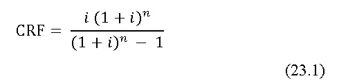
where,

          i = yearly interest rate, %

          n = life period, years.

The total annual cost of a system (TAC₁), for the pipe diameter, D₁can be written as Eq. 23.2

TAC₁ = (AC₁) _pipe + (AC₁) _pump                                                                     (23.2)

where,

          (AC₁) _pipe = annual cost of pipe line with pipe diameter D₁

          (AC₁) _pump = annual cost of pumping with pipe diameter D₁

Similarly, the total annual cost of the system (TAC₂), for the pipe diameter D₂can be written as Eq. 23.3

TAC₂ = (AC₂) _pipe + (AC2) _pump                                                 (23.3)

where,

          (AC₂) _pipe = annual cost of pipe line with pipe diameter D₂

          (AC₂) _pump = annual cost of pumping with pipediamter D₂

According to the optimal flow definition, the total annual cost of two adjacent pipe diameters will become equal at a particular flow rate. Hence, the optimal flow rate (Qc) exists between two diameters D1 and D2, the annual cost of two pipes can be equated as given in Eq.23.4.

(AC₁) _pipe + (AC₁) _pump = (AC₂) _pipe + (AC₂) _pump                                 (23.4)

In the above equation (23.4), if annual costs of pipe and pump are replaced by fixed and operating costs, then above Eq. 23.4 may be written as

(FC₁) _pipe + (OC₁) _pump = (FC₂) _pipe + (OC₂) _pump                                  (23.5)

In Eq. 23.5 the operating cost of pipe line and fixed cost of pump are not considered. The change of pipelines from D1 to D2 will have little effect on these aspects and they are considered equal in both cases.

By considering only the energy cost required towards the frictional head component of the total operating cost of the pump due to pipe diameters D1 and D2 equation 23.5 can be written as

(FC₁) _pipe +   (Q_u H₁)       C_WHP = (FC₂) _pipe +   (Q_u H₂)                                            (23.6)

                  75×3600                                     75×3600

 

                                              

 

               
                                 

  where,

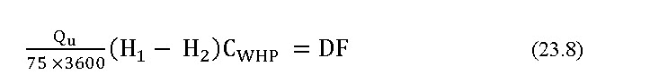
H₁ and H₂ = head losses due to friction corresponding to pipessof sizes D1 and D2 respectively,

Q_u      = total flow into the unit, L h^-1

DF     = difference in annual fixed cost per unit length of pipes D₁ and D₂, Rs.

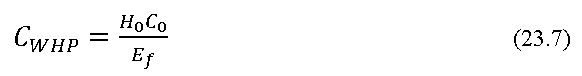
C_WHP   = cost of water horse power

H_o          = hours operating of system per year

C_o      = energy cost, Rs./bhp h

E_f       = overall pumping efficiency

Now,

                                                    

Above Eq. 23.9 can be modified further by estimating the head losses H₁ an H₂ in terms of flow taking place in the pipes by using proper friction factors for different flow regimes. Assuming the flow is in turbulent range, substitution of equation 23.10, Eq. 23.11 and Eq. 23.12 for the estimation of frictional head loss (Darcy- Weisbach formula), Reynolds number, and friction factor (Blasius formula) respectively in the above Eq. 23.9 will lead to development of Eq. 23.13.

Modified Darcy-Weisbach (DW) equation for frictional head loss is given by Eq. 23.10

H_f = 6.3755 f L Q² D^-5                                                             (23.10)

where,

          H_f      = frictional head loss, m

          f        = Darcy’s frictional factor

          L       = length of pipe, m

          Q       = flow rate, L h^-1

          D       = internal diameter of pipe, mm

The frictional head loss coefficient ‘f’ depends upon Reynolds number and the relative roughness of the pipe. Drip irrigation laterals have surface made of smooth. Flow in laterals is generally turbulent at its upstream end and becomes laminar at the downstream reach. The flow regime is characterized by Reynolds number (Re) and for cylindrical flow path this is given by

                                    

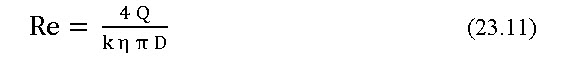
where,

          Q and D are as defined above

          k        = a constant equal to 3600

          η        = kinematic viscosity of water, m² s^-1

For turbulent flow, the Blasius equation is

f = 0.316 Re ^-0.25              (4000 > Re < 10000)                         (23.12)

 where,

          Q_C = optimal flow rate, L h^-1

Assuming that the flow through the unit is equal to optimal flow (Qu = Qc), the above equation can be converted in the following form for the calculating the optimal flow between adjacent diameters D1 and D2 as shown below.

                                 

where,

                                          

                             k₂  0.465                                                            (23.16)

Hence, the optimal flow between any two adjacent pipe diameters can be obtained by using the data on available pipe sizes in the market, their costs, bank interest rate, energy cost, hours of operation per year and overall pumping efficiency.

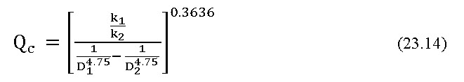
The Eq. 23.14 can be written in generalized form for different flow regimes as shown below

                                          

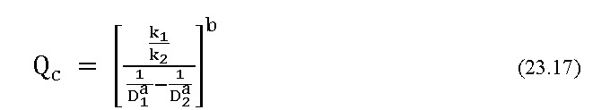
Similar derivations are made to include friction factors for laminar range, fully turbulent range and also by using Hazen-Williams equation. The resultant constants are presented in Table 23.1.

The developed equation with coefficients makes it possible to derive optimal flows between the adjacent pipe sizes available in the market. This optimal flow criterion can be used for selection of sub main and main pipe sizes required for drip irrigation.

 Table 23.1. Coefficients of optimal flow Eq. 23.17 under different flow regimes

Type of equation	Flow regime	Friction factor (Wu and Gitlin, 1973)	K2	a	b
Darcy-Weisbach (DW)	Laminar range	f = 64 Re -1.0	1.157	4.000	0.2500
	Turbulent	f = 0.316 Re -0.25	0.465	4.750	0.3636
	Fully turbulent	f = 0.130 Re-0.172	0.302	4.828	0.3506
Hazen-Williams (HW)		C = 150	0.294	4.871	0.3506

 23.2 Optimal Flows in Drip Pipes

In the present study, a model equation for determining optimal flows between adjacent pipe sizes by using both Darcy-Weisbach and Hazen-Williams equations was developed and shown in Eq. 23.17 along with its associated values was used in this section for deriving the optimal flows. The objective of this study was to find out suitable pipe sizes for sub main and main lines for drip system.

Based on available pipe sizes suitable for sub main and main lines for irrigation purpose the economical analysis has been carried out using the required input values for economical model. The input data required for deriving optimal flows between adjacent pipe sizes, annual interest rate, and life period of pipe, annual operating hours, overall pumping efficiency and energy cost. Life period of pipes vary based on pipe material. Hence, suitable value for life period should be taken considering the type of pipes used in the analysis.

The details of pipe sizes and their costs per meter length are as follows:

Pipe size, mm                  Unit cost, Rs. m^-1

          40                                   13.0

          50                                   20.5                                                            

          63                                   25.5

          75                                   36.5

          90                                   53.5

Optimal flows are derived using following assumptions:

Life period of pipe lines: 10; Annual operating hours: 2000 h; Annual interest rate :12%; Overall pumping efficiency: 65% and Energy cost is Rs. 1 bhp h (1 US$ = Rs. 55 approx.).

The optimal flows are derived for the successive sizes of the pipes under turbulent and fully turbulent range with DW equation and also with HW equation with C = 50 and shown in Fig. 23.1.

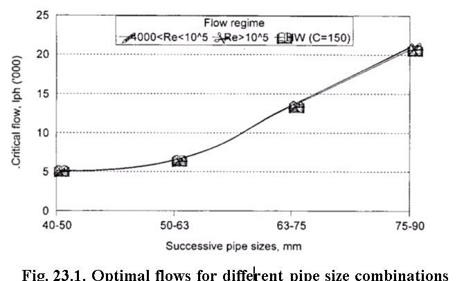  Fig. 23.1 indicates the optimal flows estimated under the three cases for turbulent range, fully turbulent range and with HW equation for C= 150 gave almost same values. With DW equation the temperature of water was considered 20⁰C. With other temperatures, incorporating suitable correction in formula will result in different optimal flows. Fig. 23.1 shows for the given criteria, the flow rate in the pipeline at which the pipe size has to be changed from one to other. By using DW equation for turbulent flow, the optimal flows for the pipe size combinations of 40-50 mm, 50-64 mm, 63-75 mm and 75-90 mm are found to be 5085, 6406, 13521 and 21049 L h^-1,respectively. These values indicate the flow rates at which pipe size has to be changed. For example, if the flow rate is expected in pipe line in between 13521 L h^-1 to 21049 L h^-1, use of 75 mm size pipe is advisable. But when, flow rate exceeds 21049 use of 90 mm pipe size will prove to be economical. This means the annual cost of 90 mm pipe size will be lower than 75 mm pipe size when flow in the pipeline is beyond 21049 L h^-1.

Hence, the optimal flow criteria will provide useful tool for making pipe size selection in the pressurized irrigation system.

23.3 Model application

The proposed theoretical developments were used for the analysis of optimal flow criteria for the pipe size selection and design of economic layouts of drip irrigation system.

23.3.1 Design of economical layouts

In this section, suitable design layouts are proposed using the computer program (Tricad) developed using optimal flow criteria for the design of drip irrigation system for a 6 ha area banana crop. Details of data used design are as follows:

Crop: banana; Spacing:2 m x 2 m; Area:6 ha (400 m x 150 m); Slope of the field:flat terrain; Soil texture:        medium textured; Peak evaporation rate:9.75 mm day^-1;Source of water:well and Static head:8 m.

Emission uniformity (EU) of greater than 90% and maximum limiting velocity in pipeline of 1.5 m s^-1 are considered as criteria for designing the drip irrigation layouts.

23.3.2 Pipe sizes for the drip system

The following pipe diameters available in the market were considered for design purpose. Data on pipe diameters and their costs are as shown in the Table 23.2. Each pipe size is designated suitably indicating its size and suitability for lateral, sub main and main.

The pipe diameters of 10 mm, 12 mm and 16 mm were considered for lateral and designated as D_l10, D_l12 and D_l16, respectively. The pipe diameters of 40 mm, 50 mm and 63 mm were considered for sub main pipes and designated as D_s40, D_s50 and D_s63, respectively. The pipe diameters of 63 mm, 75 mm and 90 mm are considered for main and designated as D_m63, D_m75 and D_m90, respectively.

Table 23.2 Pipe sizes for drip irrigation lateral, sub main and main and their respective costs

Diameter, mm	10	12	16	40	50	63	75	90
Cost, Rs. m-1	3.0	4.5	6.3	13.0	20.5	25.5	36.5	53.2
Lateral	Dl10	Dl12	Dl16
Sub main				Ds40	Ds50	Ds63
Main							Dm75	Dm90

 

 23.3.3 Planning Layout

The field size was considered as 400 m x 150 m with well located outside the boundary on the width side of the field as shown in the layout (Fig. 23.2).

Based on water requirement estimates for the crop, it was considered to provide one 4 l h^-1 emitter for each plant. The total number of plants in 6 ha field is estimated to be 14,800 by leaving one row space at the centre along the length for easy operation of subunits. Based on emitter discharge and number of plants in the field, the pump discharge requirement is computed to be 59,200 L h^-1. This flow in the main line of D_m90 will cause the flow velocity of 2.59 m s^-1, which was considered to be high for irrigation pipe lines,and also it would cause the requirement of bigger size prime mover for operating the pump. In order to use specified pipe diameter to D_m90, D_m75 and D_m63 for the main and also to reduce the pump capacity and prime mover requirement, it is desired to irrigate field in two shifts. For this reason, the field needs to be divided into two halves for irrigation purpose. This aspect has been considered while planning irrigation layouts.

The proposed layout consists of subunits with laterals on one side of the sub main. The field is divided into eight subunits with four on each side of main line. The length of sub main is 75 m with 37 rows and with 50 emission points on each row. The subunits are numbered serially from 1 to 8 as shown in Fig 23.2.

F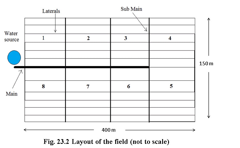

 

23.3.4 Irrigation Plans

The field shown in layout (Fig 23.2) can be irrigated in through two different plans as shown in Table 23.3.

Table 23.3 irrigation plants for layout proposed

Irrigation plan	Description
I1	Irrigating subunits 1,2,3, and 4 in one shift and 5,6,7, and 8 in another shift
I2	Irrigating subunits 1, 2, 7 and 8 in one shift and 3, 4, 5 and 6 in another shift

 

23.3.5 Design of Main Pipe Lines

Design of main pipes was made based on both optimal flow criteria and velocity limit in the main line.

23.3.5.1 Based on optimal flow criteria

In order to design main line pipe sizes for laying in field the optimal flow rates were computed for the successive pipe sizes to be considered for main line sizes. In estimating the optimal flows, the following assumptions were made.

Life period of pipes, n:10 years; Interest rate, i:12%; Energy cost/bhp h:Rs. 1.00; Operating hours per annum:2000 h and Overall pumping efficiency:  65%

In order to study the effect of time of operation on optimal flows, the analysis was made for the operating hours from 500 to 2500 at an interval of 500 hours. The optimal flows estimated are shown in Table 23.4.

Table 23.4 indicates the flow rates at which the pipe diameters are to be changed from lower to higher sizes for the consequent pipe sizes of 63-75 mm and 75-90 mm for different annual hours of operation. For, example at 2000 hours of operation, the pipe size required to be changed from 63 mm to 75 mm when the flow in the network exceeds 13,520 L h^-1 and similarly, the pipe size need to be changed from 75 mm to 90 mm at 21,048 L h^-1.

Table 23.4 Optimal flows for pipe size combinations of 63-75 mm and 75-90   mm for different operating hours in a year

Operating hours	63-75 mm		75-90 mm
	Lh-1	L s-1	L h-1	L s-1
500	22382	6.217	34843	9.678
1000	17396	4.832	27081	7.522
1500	15011	4.120	23369	6.491
2000	13520	3.756	21048	5.847
2500	12467	3.463	19408	5.391

 

Table 23.4 indicates the flow rates at which the pipe diameters are to be changed from lower to higher sizes for the consequent pipe sizes of 63-75 mm and 75-90 mm for different annual hours of operation. For, example at 2000 hours of operation, the pipe size required to be changed from 63 mm to 75 mm when the flow in the network exceeds 13,520 L h^-1 and similarly, the pipe size need to be changed from 75 mm to 90 mm at 21,048 L h^-1.

23.3.5.2 Velocity Limit in the Main Pipe

An attempt has also been made to design the size of main pipe keeping the velocity limit as 1.5 m s^-1 (ASAE, 1991). In order to select suitable pipe size for the expected flow rates and corresponding velocity is worked ( Table 23.5). Table 23.5 is referred while applying the velocity criteria in selection of main pipe.

Table 23.5. Flow velocities in the main pipeline for different diameters at various flow rates

Expected flow, L h-1	Velocity in different main line pipe sizes, m s-1
	63 mm	75 mm	90 mm
7400	0.66	0.47	0.32
14800	1.32	0.93	0.65
22200	1.98	1.40	0.97
29600	2.64	1.86	1.29
59200	5.28	3.72	2.59

 

23.3.6 Estimation of Main Line Pipes

With the help of Tables 23.4 and 23.5 and considering the layout and expected flows in the main line in different zones, the requirement of the main pipelines was worked out and presented in Table 23.6 for different irrigation plans.

In calculating the pipe sizes the maximum flow expected in each zone was considered. It was also assumed that the water source was 10 m away from the field boundary. Hence, 10 m length of the pipe was added to the segment at the beginning to arrive at the final estimates of length of pipe and cost.

It is clear from the Table 23.6 that there are significant differences in the estimates of pipe lines in the two irrigation plans. With optimal flow criteria in case of irrigation plan I₁, the requirement of the pipe were 100 m of 63 mm size, 100 m of 75 mm size and 110 m of 90 mm size. With I₂ plan, the requirement of the pipes was 100 m of 75 mm and 210 m of 90 mm. The estimates were obtained based on the flow expected in each segment of the pipe. For example, in case of I₁, considering the subunits 1, 2, 3 and 4 are irrigated in one shift, the main pipeline feeding the subunit 4 should carry the flow of 7,400L h^-1 and accordingly 63 mm pipe size was found suitable. Similarly, the segment supplying water to 3 and 4 subunits will carry 14,800 L h^-1 and need 75 mm pipe size of 100 m length, then the pipe segment carrying flow to 2, 3 and 4 sub units should carry 22,200 l h^-1 and require 90 mm size of 100 m length. Then the segment, which has to carry flow for all the subunits at the rate of 29,600 L h^-1, will be of 90 mm size and 10 m length. In the similar way estimates were made for I₁ assuming that 3, 4, 5 and 6 subunits are to be irrigated in one shift. The segment of pipe carrying water to the subunits 4 and 5 should carry 14,800 L h^-1 and should be of 75 mm and 100 m length. Then for entire area under subunits 3, 4, 5 and 6 the total flow; requirement was 29,600 L h^-1 and the pipe size should be of 90 mm of 210 m lengths. The cost of the main line under 11 and 12 were found to be Rs. 12,052 and Rs. 14822 respectively. It shows net saving of Rs. 2,770 was possible by adopting I₁ over I₂. This indicates that the selection of irrigation pipe is an important aspect to optimize the pipe requirement. Similarly, main lines estimates were made by considering the velocity criteria. Estimates were also made based on the assumption that uniform size pipes could be used as main lines. By considering the initial investment on the pipeline, the pipe sizes selected based on velocity criteria were found to be less expensive than those selected under optimal flow criteria.

Table 23.6 Estimates of length of pipe line (m) required for main based on optimal flow criteria and velocity limit

Irrigation plan	Optimal flow criteria				Velocity limit criteria
	63 mm	75 mm	90 mm	Total cost, Rs.	63 mm	75 mm	90 mm	Total cost, Rs.
I1	100	100	110	12052	200	100	10	9282
I2		100	210	14822	100		210	13722

23.3.7 Comparison of Irrigation plans in terms of Main Pipe Selection

In order to compare the economics of pipe size selection for main line, the pipes sizes D_m63, D_m75 and D_m90 were also considered for mainlines separately without any sizing. The frictional head loss in the mainline for different pipe sizes is estimated by considering the amount of flow taking place in each zone. The details of the comparisons on frictional head loss and annual costs are presented in the Table 23.7.

Table 23.7 furnishes the detailed calculations of the frictional head loss in the main, energy cost to overcome friction, annual fixed costs and the horsepower requirement for the prime mover for all the criteria under which the main size was selected. The annual fixed cost on the main line was more for larger pipe sizes. However, the annual operating cost in order to overcome the friction was less. The total annual costs are considered for purpose of comparisons. The pipe size combinations with lower annual cost are better for selection. In all irrigation plans the optimal flow criteria proves to be more economical. In calculating the hp requirement, a constant loss of 2 m of head in accessories and 8 m static suction head were considered. Considering the pressure head at the inlet of the subunit as 10 m, the total head requirement estimated to be 20 m plus the frictional head loss in the main line as presented in the Table 23.7.

In all the cases the optimal flow criteria proves to be requiring less horsepower to operate the prime mover than with uniform sizes of D_s63 and D_s75. However use of uniform size of D_s90would need less prime mover size, but the annual cost of the pipeline would be much higher than those selected with optimal flow criteria. This shows the optimal flow criteria should be the basis for pipe size selection in selection of the main line in drip irrigation systems design.

 Table 23.7 Comparison of different irrigation plans based on mainline pipes Selection.

Irrigation plan	Pipe sizes for main as per	Frictional head loss, (Hf), m	Energy cost due to Hf, Rs	Annual fixed cost of the main, Rs.	Total annual cost, Rs.	hp of the prime mover
I1	Optimal flow	3.06	560.3	2401.2	2961.5	3.89
	Velocity	5.88	1150.2	1849.3	2999.5	4.36
	63 mm	9.61	2152.8	1575	3727.8	4.99
	75 mm	4.19	939.3	2254.4	3193.7	4.08
	90 mm	1.77	395.6	3285.9	3681.5	3.67
I2	Optimal flow	4.54	1139.6	2953.1	4292.7	4.14
	Velocity	6.02	1588.8	2734	4322.8	4.39
	63 mm	21.12	6682.7	1575	8257.8	6.94
	75 mm	9.23	2919.5	2254.4	5173.9	4.93
	90 mm	3.88	1228.6	3285.9	4487.4	4.03

 23.4 Summary

Optimal flow criterion and Life Cycle Costing (LCC) techniques were used for development of an equation for economic pipe size selection. The model equation developed was based on both economic and as well as hydraulic considerations. It estimates the flow rate at which the designer should change from one size to another size pipes. The main line selection made for 6 ha banana plot was compared with other methods of pipe selection. Application of the optimal flow method resulted in lowest annual cost of mainlines in comparison to the selection on velocity basis and uniform size pipes. In all irrigation plans the optimal flow criteria proved to be more economical.

References

• ASAE (1991). Design Installation and Performance of Underground Thermoplastic Irrigation Pipe Line. ANSI/ASAE standard, S376.1.

• James, L. D and R. R. Lee (1971).Economics of Water Resources Planning. McGraw Hill, Bombay and New Delhi, India.

• Keller, J (1965). Selection of Economical Pipe Sizes for Sprinkler Irrigation Systems. Transactions of ASAE, 8(2):186-190.

• Mohatar, R. H. (1985). A Model for Design of Optimization of Branched-pipe Networks. M.Sc. Thesis, the American University of Beirut, Beirut, Lebanon

• Reddy, K. Y. and Tiwari, K. N., 2006. Economical Pipe Size Selection Based on Optimal Flow. International Agricultural Engineering Journal, 15(2-3): 109-121.

Suggested Reading

• Bagley, J. M. and R. K. Linsley (1961).Graphical determination of the most economical pipe size. Agricultural Engineering, 42(10):550-551.

• Hathoot, H. M (1984). Minimum cost design of pipelines. J. Transp. Engg. ASCE, 112(2):465-480.

• Hathoot, H. M (1986). Minimum cost design of horizontal pipelines. J. Transp. Engrg, ASCE, 110(3):382-389.