Remote Sensing & GIS Applications

Lesson 12 Image Classification

12.1 Supervised Classification

In this technique, the image is classified on the priori knowledge of the analyst. The image is classified on the basis of predefined landuse-landcover classes and algorithm by the analyst. At first, the analyst must have some knowledge about the landuse-landcover classes of the study area; on this basis the landuse-landcover classes will be defined. There are three basic steps in supervised classification process. First is the training stage, in which representative sample sites of known feature types are collected, which is termed as training sites or signature class depending on the spectral response patterns of the features which we can identify from image or from other sources like aerial photography, ground truth data, personal experience, previous studies, or maps. In the second or classification stage, the unknown pixels of image are compared to the spectral patterns with the training sites and they are assigned to a class as defined by some algorithm. The third is the output presentation in the form of maps, table of area data and digital data files.

After the signatures are collected, the pixels are sorted into classes based on the algorithms used. The algorithms used in supervised classification are: a) Minimum Distance to Mean, b) Parallelepiped, c) Gaussian Maximum Likelihood.

a) Minimum Distance to Mean Classifier: The minimum distance to mean classifier is simplest mathematically and very efficient in computation. In this procedure the DN value of the training sets are plotted in a scatteromgram. Here a 2D scatteromgram is drawn for an example shown through Fig. 12.1. DN values of five training sets are plotted and their means are computed (shown with a subscript). Now a unknown pixel A will be classified or be assigned to a class by a distance calculation from the mean of each class to the pixel A. This is why this algorithm is named as minimum distance to mean classifier. Therefore the pixel A will be assigned to the class whose mean value is nearest to A. In this example, the unknown pixel A will be assigned to the sand class. This way the pixels of entire image are assigned to different landuse landcover classes. Thus for an n-Dimensional multispectral data, n-D scatter diagram is plotted; the mean of each classes are calculated and the image is classified according to the shortest distance class. The most used distance calculation method is Euclidean distance formulated as below:

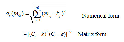
where,

          nb= number of bands

          j= a particular band

          i= a particular class

          k_j = DN value of pixel at band j

          C_ij =mean of DN values in band j for the sample for class i

          d_e (C_ik) = Euclidean distance from the mean of a class to any unknown pixel

          T = transposition function

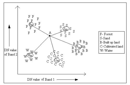
Fig. 12.1. Minimum distance to means classification strategy.

b) Parallelepiped Classifier: The parallelepiped classification strategy is also computationally simple and efficient. As an example, the DN values of two bands are plotted in a scatter diagram in the similar way to minimum distance to mean classifier. In this procedure a rectangular box is fitted for each class defined by the maximum and minimum values of each bands shown in Fig. 12.2. Now the classification of the pixels depends on whether any pixel falls inside any rectangular box (or parallelepiped decision region) or not. If the pixel falls inside the parallelepiped, it is assigned to the class. However, if the pixel falls within more than one class, it is put in the overlap class. If the pixel does not fall inside any class, it is assigned to the null class. In the given example, three unknown pixels are taken (A, B, and C). The pixel A will assigned to the water class, as it falls in parallelepiped of water class; whereas pixel B will be labeled as unknown class and the pixel C will labeled as overlap class. Overlap is caused due to high correlation or covariance between bands. Covariance is the tendency of spectral values to vary similarly in other bands. This method is poor as the spectral response patterns are frequently highly correlated and high covariance.

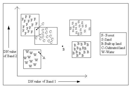
Fig. 12.2. Parallelepiped classification strategy.

c) Gaussian Maximum Likelihood Classifier: The maximum likelihood classifier is one of the most popular methods of classification in remote sensing, in which a pixel with the maximum likelihood is classified into the corresponding class. In this method it is assumed that the training sets of each class of each band have the normal distribution, which is Gaussian in nature and can be described by the mean vector and covariance matrix. From this information, the statistical probability is computed for a given pixel value being a member of a particular landuse landcover class. The probability is calculated for an unknown pixel for each class of the training sets. As an example, in the Fig. 12.3, the probability values for band 1 for the mean of the classes (A and B) and unknown pixel X is plotted in 2D graph. The bell-shaped curves are called probability density functions. In the example, it is found that the probability of the unknown pixel X for being in class B is greater than class A. So, the pixel X will be labeled as class B. The probability density functions are used to classify unidentified pixels by computing the probability of the pixels values belonging to each category. Thus it takes large number of computations to classify an image and is much slower in computation than the previous methods.

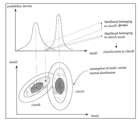
Fig. 12.3. Concept of maximum likelihood classification method.

(Source:stlab.iis.u-tokyo.ac.jp/~wataru/lecture/rsgis/rsnote/cp11/cp11-7.htm)

12.2 Unsupervised Classification   

In supervised classification, the image pixels are categorized as defined by the analyst specified landuse landcover classes and an algorithm thereafter. In contrast to supervised classification, in unsupervised classification an algorithm is first applied to the image to form some spectral classes (clusters); thereafter the image is classified based on these classes. Then the analyst tries to assign spectral classes to desirable information classes or landuse landcover classes. The spectral classes in an image may be numerous; it is difficult to obtain all of them as training areas in supervised classification, but in the unsupervised approach, they are found automatically. Unsupervised classified image must be compared with some reference data to identify the spectral classes which is automatically generated.

One of the commonly used algorithms of unsupervised classification is the “K-means” clustering method. It is an iterative method. The number of output cluster or spectral classes (assume k clusters) is specified by the analyst. The algorithm locates the centroids of k clusters in the multidimensional data. Each pixel in the image is assigned then to its nearest cluster. At this point the mean of each clusters re-calculated using the result obtained from the previous step. The image then reclassified using the revised mean of each clusters. This procedure continues until there is no significant change in the location of cluster mean vector between successive iterations.

The K-means algorithm is composed of the following steps:

1. Place K points into the space represented by the objects that are being clustered. These points represent initial group centroids.

2. Assign each object to the group that has the closest centroid.

3. When all objects have been assigned, recalculate the positions of the K centroids.

4. Repeat Steps 2 and 3 until the centroids no longer move in centroids.

One more useful algorithm in unsupervised classification is ISODATA algorithm. The ISODATA algorithm is similar to the k-means algorithm with the distinct difference that the ISODATA algorithm allows for different number of clusters while the k-means assumes that the number of clusters is known a priori. In ISODATA algorithm, clusters are merged if either the number of members (pixel) in a cluster is less than a certain threshold or if the centers of two clusters are closer than a certain threshold. Clusters are further split into two different clusters if the cluster standard deviation exceeds a predefined value and the number of members (pixels) is twice the threshold for the minimum number of members.

12.3 Fuzzy Classification

In remote sensing imagery, spectral reflectance/radiance of more than one features are recorded in one pixel. Thus one pixel contained information more than one feature. These pixels are known as mixed pixel. In case classifying an image contains mixed pixel, the mix pixels is a member in more than one class. Therefore, it requires a fuzzy logic based model to solve the unmixing problem in classification. Fuzzy classification and spectral mixture classification are two commonly used techniques.

There are many approaches of fuzzy classification, one most important technique is fuzzy c-means. Fuzzy c-means is similar to K-means clustering. In fuzzy c-means technique, fuzzy regions are formed between the boundaries of the clusters generated in K-means clustering. The fuzzy-ness (possibility of one pixel to be member of more than one class) of image pixels can be presented or a membership grade value assigned describes how close is a pixel to the means of the classes.

Keywords: Classification, Supervised, Maximum likelihood, Parallelepiped, Minimum distance to mean, Unsupervised, K-means, ISODATA, Fuzzy.

References

stlab.iis.u-tokyo.ac.jp/~wataru/lecture/rsgis/rsnote/cp11/cp11-7.htm

Suggested Reading

• Bhatta, B., 2008, Remote sensing and GIS, Oxford University Press, New Delhi, pp. 353-369.

• Joseph, G., 2005, Fundamentals of remote sensing, Universities Press (India) Private Limited, pp. 134-142.

• Lillesand, T. M., Kiefer, R. W., 2002, Remote sensing and image interpretation, Fourth Edition, pp. 532-565.

• www.cs.ubbcluj.ro/~studia-i/2007-1/09-Gavris.pdf