Remote Sensing & GIS Applications

Lesson 13 Classification Accuracy Assessment

• Classification Error Matrix

One of the most common means of expressing classification accuracy is the preparation of a classification error matrix (confusion matrix or contingency table). To prepare a error matrix first task is to locate ground reference test pixels or sample collection, based on which an error matrix is formed. There are many mathematical approaches in this regard. Generally it is suggested that a minimum of 50 samples of each landuse landcover classes should be included. If the study area is large or the numbers of landuse landcover classes are more than 12, the sample should be 75 to 100. Data sampling can be done using various procedures such as: random, systematic, stratified random, stratified systematic unaligned, and cluster.  An error matrix compares the relationship between known reference data (ground data) and the corresponding results obtained from classification.

Table 13.1 is an error matrix obtained from a data analysis (Randomly sample test pixels) and Table 13.2 presents results of various accuracy measurements.

Table 13.1 Error Matrix resulting from a data analysis

Classification Data	Water	Sand	Forest	Urban	Cultivated land	Barren land	Row Total
Water	150	12	0	0	0	0	162
Sand	0	56	0	10	0	0	66
Forest	0	0	130	0	17	0	147
Urban	0	0	0	126	0	15	141
Cultivated land	0	0	20	0	78	12	110
Barren land	0	0	5	24	15	115	159
Column Total	150	68	155	160	110	142	785

 

Table 13.2 Different measurement from error matrix

Omission error	Producer’s Accuracy	Commission error	User’s Accuracy
Water=0/150=0%	Water=150/150=100%	Water=12/162=7%	Water=150/162=93%
Sand=12/68=18%	Sand=56/68=82%	Sand=10/66=15%	Sand=56/66=85%
Forest=25/155=16%	Forest=130/155=84%	Forest=17/147=12%	Forest=130/147=88%
Urban=34/160=21%	Urban=126/160=79%	Urban=15/141=11%	Urban=126/141=89%
Cultivated land =32/110=29%	Cultivated land =78/110=71%	Cultivated land =32/110=29%	Cultivated land =78/110=71%
Barren land =27/142=19%	Barren land =115/142=81%	Barren land =44/159=28%	Barren land =115/159=72%
Overall accuracy=(150+56+130+126+78+115)/785=83%

From the error matrix several measures of classification accuracy can be calculated using simple descriptive statistics (Table 13.2) as discussed below:

(a)   Omission error

(b)   Commission error

(c)    Overall accuracy

(d)   Producer’s accuracy

(e)    User’s accuracy

(f)    Kappa coefficient (k)

(a) Omission error (exclusion): represent pixels that belong to the actual class but fail to be classified into the actual class (e.g., 12 pixels which should be classified as sand but classified as water).

(b) Commission error (inclusion): represents the pixels that belong to another class but are classified to a class (e.g., 20 pixels of forest class and 12 pixels of barren land class included in cultivated land).

(c) Overall accuracy: represents the total classification accuracy. It is obtained by dividing the total numbers of correctly classified pixels by the total numbers of reference pixels. The drawback of this measure is that it does not tell us about how well individual classes are classified. The producer and user accuracy are two widely used measures of class accuracy depends on the omission and commission accuracy respectively.

(d) Producer’s accuracy: it refers to the probability that a certain feature of an area on the ground is classified as such. It results from dividing the numbers of pixels correctly classified in each category by the numbers of sample pixels taken for this category (column total).

(e) User’s accuracy: it refers to the probability that a pixel labeled as a certain class in the map is really this class. It is obtained by dividing the accurately classified pixels by the total numbers of pixels classified in this category. The producer accuracy and user accuracy are not same typically. For example, the producer accuracy of water is 100% whereas the user accuracy is 93%.

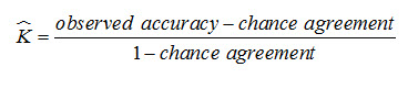
(e) Kappa coefficient (): it is a discrete multivariate method of use in accuracy assessment. In classification process, where pixels are randomly assigns to classes will produce a percentage correct value. Obviously, pixels are not assigned randomly during image classification, but there are statistical measures that attempt to account for the contribution of random chance when evaluating the accuracy of a classification. The resulting Kappa measure compensates for chance agreement in the classification and provides a measure of how much better the classification performed in comparison to the probability of random assigning of pixels to their correct categories.

is theoretically expressed as:

The can be calculated as:

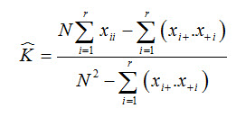
where,

          r = the number of rows in the error matrix

          x_ii = the number of observations in the row i and column i

          x_i+ = total of observations in row i

          x_+I = total of observations in column i

          N = total number of observations included in matrix

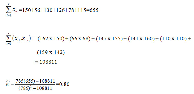
A value of 0.80 implies that the classification process was avoiding 80% of the errors that a completely random classification would generate.

13.2 Data Merging

Image acquisition by a remote sensing sensor of an area of study can be available in the following cases:

• Image acquired by different sensors;

• Image acquired by same sensor operating at different spectral bands;

• Image acquired by same sensor at different time;

• Image acquired by same sensor at different polarization.

In many applications it may be required to merge multiple data sets covering same geographical area. Data merging operation generally can be categorized as: multi-temporal data merging, multi-sensor image merging, and multi-polarization image merging.

Multi-temporal data merging: The term multi-temporal refers to the repeated imaging of an area over a time period. By analyzing an area through time, it is possible to develop interpretation techniques based on an object’s temporal variations, and to discriminate different pattern classes accordingly. Multitemporal data merging is combining images of the same area taken on different time, depending on the nature of purpose. The principal advantage of multitemporal analysis is the increased amount of information for the study area. The information provided for a single image is, for certain applications, not sufficient to properly distinguish between the desired pattern classes. This limitation can sometimes be resolved by examining the pattern of 2 temporal changes in the spectral signature of an object. This is particularly important for vegetation applications (source: heim.ifi.uio.no/inf5300/2008/datafusion_paper.pdf).

For example, agricultural crop interpretation is often facilitated through merger of images taken early and late in the growing season. In early season images in the upper Midwest, bare soils often appear that late will probably be planted in such crops perennial alfalfa or winter wheat in an advanced state of maturity. In the late season images, substantial changes in the appearance of the crops present in the scene are typical. Merging various combinations of bands from the two dates to create color composites can aid the interpreter in discriminating the various crop types present (Lillesand & Kiefer, 2000).

Multi-sensor data merging: Each sensor has its own characteristics. Depending on the nature of application, images obtained from different sensors can be merged, which requires different preprocessing. The image merging or fusion of two images obtained from multispectral image r (MSI) and hyperspectral imager (HSI) are shown in Fig. 13.1. Multispectral imager generally has high spatial resolution and low spectral resolution; whereas hyperspectral imager has low spatial resolution but high spectral resolution. Image fusion taken from these two sensors can be of both high spectral and spatial resolution.

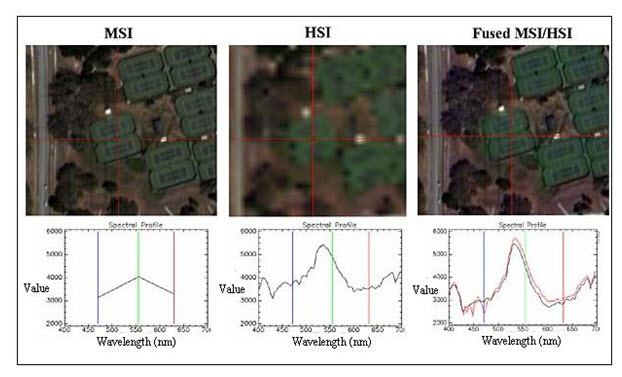
Fig. 13.1. Multisensor image fusion (merge).

(Source: www.weogeo.com/blog/Image_Fusion_and_Sharpening_With_Multi_and_Hyperspectral_Data.html)

Multipolarization image merging:  Multipolarization image merging is related to microwave image data, refers to image merging of different polarization.

13.3   GIS Integration

GIS integration refers to combining data of different types and from different sources. In a digital environment, where all the data sources are geometrically registered to a common geographic base, the potential for information extraction is extremely wide. This is the concept for analysis within a digital GIS database. The integration with GIS allows a synergistic processing of multisource spatial data.

Any data source which can be referenced spatially can be used in this type of environment. A DEM/DTM is just one example of this kind of data. Other examples could include digital maps of soil type, land cove classes, forest species, road networks, and many others, depending on the application. The results form a classification of a remote sensing data set in map format could also be used in a GIS another data source to update existing map data.

As an example, GIS is now being widely used in crop management. Remote sensing and GIS have made huge impacts on how those in the agricultural planners are monitoring and managing croplands, and predicting biomass or yields. Map products, derived from remote sensing are usually critical components of a GIS. Remote sensing is an important technique to study both spatial and temporal phenomena (monitoring). Through the analysis of remotely sensed data, one can derive different types of information that can be combined with other spatial data within a GIS.

The integration of the two technologies creates a synergy in which the GIS improves the ability to extract information from remotely sensed data, and remote sensing in turn keeps the GIS up-to-date with actual environmental information.

As a result, large amounts of spatial data can now be integrated and analysed. This allows for better understanding of environmental processes and better insight into the effect of human activities. The GIS and remote sensing can thus help people to arrive at informed decisions about their environment. Like in all models, however, both maps and thematic data are abstractions or simplifications of the real world. Therefore, GIS and remote sensing can complement, but never completely replace field observations, (Bhatta, 2008).

Keywords: Accuracy assessment, Error matrix, Kappa statistics, Data merging, GIS integration.

References

• Bhatta, B., 2008, Remote sensing and GIS, Oxford University Press, New Delhi, pp.381.

• heim.ifi.uio.no/inf5300/2008/datafusion_paper.pdf

• Lillesand, T. M., Kiefer, R. W., 2002, Remote sensing and image interpretation, Fourth Edition, pp.576.

Suggested Reading

• heim.ifi.uio.no/inf5300/2008/datafusion_paper.pdf

• www.utsa.edu/lrsg/Teaching/EES5083/L9-ClassAccuracy.pdf

• www.weogeo.com/blog/Image_Fusion_and_Sharpening_With_Multi_and_Hyperspectral_Data.html

• www.yale.edu/ceo/OEFS/Accuracy_Assessment.pdf