Remote Sensing & GIS Applications

Lesson 23 Projection System

  

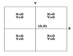
Fig. 23.1. The signs of x- and y-coordinates in a projected coordinate system. (Source: ESRI Map projections.pdf)

23.1.1 Map projection

A map projection is used to portray all or part of the round Earth on a flat surface. This cannot be done without some distortion.

(http://rnlnx635.er.usgs.gov/mac/isb/pubs/MapProjections/projections.html). Whether you treat the earth as a sphere or a spheroid, you must transform its three-dimensional surface to create a flat map sheet.

One easy way to understand how map projections alter spatial properties is to visualize shining a light through the earth onto a surface, called the projection surface. Imagine the earth's surface is clear with the graticule drawn on it. Wrap a piece of paper around the earth. A light at the center of the earth will cast the shadows of the graticule onto the piece of paper. You can now unwrap the paper and lay it flat. The shape of the graticule on the flat paper is different from that on the earth. The map projection has distorted the graticule.

A map projection uses mathematical formulas to relate spherical coordinates on the globe to flat, planar coordinates. Different projections cause different types of distortions. Some projections are designed to minimize the distortion of one or two of the data's characteristics. A projection could maintain the area of a feature but alter its shape. In the graphic below, data near the poles is stretched. (ESRI Map projections.pdf)

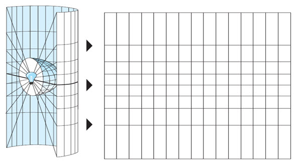
Fig. 23.2. The graticule of a geographic coordinate system is projected onto a cylindrical projection surface. (Source: Kennedy, 1994)

23.1.2 Major map projections

The three major types of projections developed from this method are the:

(1) Conic

(2) Planar

(3) Cylindrical

(1) Conic projections

Conic projections, points from the globe graticule are transferred to a cone which has been enveloped around the sphere. The cone is then unrolled into a flat plane. The normal aspect is the north or south pole where the axis of the cone (the point) coincides with the pole. Conic projections can only represent one hemisphere, or a portion of one hemisphere, for the cone does not extend far beyond the center of the sphere. Conic projections are often used to project areas that have a greater east-west extent than north-south, e.g., the United States. When projected from the center of the globe, the typical grid appearance for Conic projections shows parallels forming arcs of circles facing up in the Northern Hemisphere and down in the Southern Hemisphere; and meridians are either straight or curved and radiate outwards from the direction of the point of the cone. (Laurie A. B. Garo, 1997, Introduction to Map Projections).

The most simple conic projection is tangent to the globe along a line of latitude. This line is called the standard parallel. The meridians are projected onto the conical surface, meeting at the apex, or point, of the cone. Parallel lines of latitude are projected onto the cone as rings. The cone is then ‘cut’ along any meridian to produce the final conic projection, which has straight converging lines for meridians and concentric circular arcs for parallels. The meridian opposite the cut line becomes the central meridian.

Conic projections are used for mid latitude zones that have an east-to-west orientation. Somewhat more complex conic projections contact the global surface at two locations. These projections are called secant conic projections and are defined by two standard parallels. It is also possible to define a secant projection by one standard parallel and a scale factor. The distortion pattern for secant projections is different between the standard parallels than beyond them. Generally, a secant projection has less overall distortion than a tangent case. On still more complex conic projections, the axis of the cone does not line up with the polar axis of the globe. These are called oblique. (ESRI Map projections.pdf)

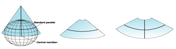
Fig. 23.3. (a) Tangent conic projection. (Source: www.arcgis.com)

With the tangent case Fig. 3(a), A cone is placed over a globe. The cone and globe meet along a latitude line. This is the standard parallel. The cone is cut along the line of longitude that is opposite the central meridian and flattened into a plane.

In secant case Fig. 3(b), A cone is placed over a globe but cuts through the surface. The cone and globe meet along two latitude lines. These are the standard parallels. The cone is cut along the line of longitude that is opposite the central meridian and flattened into a plane.

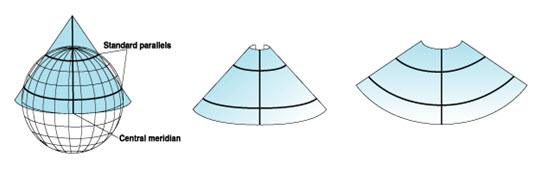
Fig. 23.3. (b) Secant conic projection. (Source: www.arcgis.com)

The representation of geographic features depends on the spacing of the parallels. When equally spaced, the projection is equidistant in the north–south direction but neither conformal nor equal area such as the Equidistant Conic projection. For small areas, the overall distortion is minimal. On the Lambert Conic Conformal projection, the central parallels are spaced more closely than the parallels near the border, and small geographic shapes are maintained for both small-scale and large-scale maps. Finally, on the Albers Equal Area Conic projection, the parallels near the northern and southern edges are closer together than the central parallels, and the projection displays equivalent areas (Kennedy, 1994).

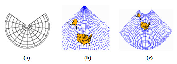
Fig. 23.4. (a) Equidistant conic, (b) Lambert Conformal Conic Projection, and (c) Albers Equal Area Conic projection.

(Source: http://www.progonos.com/furuti/MapProj/Normal/ProjTbl/projTbl.htm and Class notes on Map projection)

(2) Cylindrical projections

Cylindrical projections are formed by wrapping a large, flat plane (e.g., a large sheet of paper) around the globe to form a cylinder. The points on the spherical grid are transferred to the cylinder which is then unfolded into a flat plane. The equator is the "normal aspect" or viewpoint for these projections.

This family of projections are typically used to represent the entire world. When projected from the center of the globe with the normal aspect, the typical grid appearance for cylindrical projections shows parallels and meridians forming straight perpendicular lines. The spacing varies depending on the type of cylindrical projection. (Laurie A. B. Garo, 1997, Introduction to Map Projections).

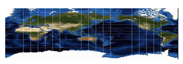
Fig. 23.5. This is an example of a cylindrical map projection and it is one of the most famous projections ever developed.  It was created by a Flemish cartographer and geographer – Geradus Mercator in 1569.  It is famous because it was used for centuries for marine navigation.  The sole reason for this is that any line drawn on the map was a true direction.  However, shapes and distances were distorted.  Notice the huge distortions in the Arctic and Antarctic regions, but the reasonable representation of landmasses out to about 50° north and south. (Source: www.icsm.gov.au)

Cylindrical projections can also have tangent or secant cases. The Mercator projection is one of the most common cylindrical projections, and the equator is usually its line of tangency. Meridians are geometrically projected onto the cylindrical surface, and parallels are mathematically projected, producing graticular angles of 90 degrees. The cylinder is ‘cut’ along any meridian to produce the final cylindrical projection. The meridians are equally spaced, while the spacing between parallel lines of latitude increases toward the poles. This projection is conformal and displays true direction along straight lines. Rhumb lines, lines of constant bearing, but not most great circles, are straight lines on a Mercator projection. (Kennedy, 1994).

For more complex cylindrical projections the cylinder is rotated, thus changing the tangent or secant lines. Transverse cylindrical projections such as the Transverse Mercator use a meridian as the tangential contact or lines parallel to meridians as lines of secancy. The standard lines then run north and south, along which the scale is true. Oblique cylinders are rotated around a great circle line located anywhere between the equator and the meridians. In these more complex projections, most meridians and lines of latitude are no longer straight. of equidistance. Other geographical properties vary according to the specific projection.

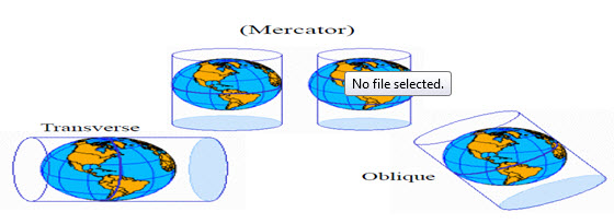
Fig. 23.6. A cylinder is placed over a globe. The cylinder can touch the globe along a line of latitude (normal case or Mercator), a line of longitude (transverse case), or another line (oblique case).

(Source: Class notes on Map Projection)

The National Imagery and Mapping Agency (NIMA) (formerly the Defense Mapping Agency) adopted a special grid for military use throughout the world called the Universal Transverse Mercator (UTM) grid.

(egsc.usgs.gov/isb/pubs/factsheets/fs07701.html).

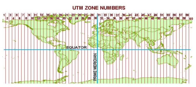
Fig. 23.7. Universal Transverse Mercator system.

(Source: www.luomus.fi/english/botany/afe/map/utm_ups.pdf)

The UNIVERSAL TRANSVERSE MERCATOR is also very widely used. In this grid, the world is divided into 60 north-south zones, each covering a strip 6° wide in longitude. These zones are numbered consecutively beginning with Zone 1, between 180° and 174° west longitude, and progressing eastward to Zone 60, between 174° and 180° east longitude. Thus, the conterminous 48 States are covered by 10 zones, from Zone 10 on the west coast through Zone 19 in New England (fig.7). In each zone, coordinates are measured north and east in meters. (One meter equals 39.37 inches, or slightly more than 1 yard.) The northing values are measured continuously from zero at the Equator, in a northerly direction. To avoid negative numbers for locations south of the Equator, NIMA's cartographers assigned the Equator an arbitrary false northing value of 10,000,000 meters. A central meridian through the middle of each 6° zone is assigned an easting value of 500,000 meters. Grid values to the west of this central meridian are less than 500,000; to the east, more than 500,000.

(egsc.usgs.gov/isb/pubs/factsheets/fs07701.html).

(3) Planar or Azimuthal Projection

 Azimuthal projections, the spherical (globe) grid is projected onto a flat plane, thus it is also called a plane projection. The poles are the "normal aspect" (the viewpoint or perspective) which results in the simplest projected grid for this family of projections. That is, the plane is normally placed above the north or south pole. Normally only one hemisphere, or a portion of it, is represented on Azimuthal projections. When projected from the center of the globe with the normal aspect, the typical grid appearance for Azimuthal projections shows parallels forming concentric circles, while meridians radiate out from the center. (Laurie A. B. Garo, 1997, Introduction to Map Projections).

Planar projections project map data onto a flat surface touching the globe. This type of projection is usually tangent to the globe at one point but may be secant. The point of contact may be the North Pole, the South Pole, a point on the equator, or any point in between. This point specifies the aspect and is the focus of the projection. The focus is identified by a central longitude and a central latitude. Possible aspects are polar, equatorial, and oblique.

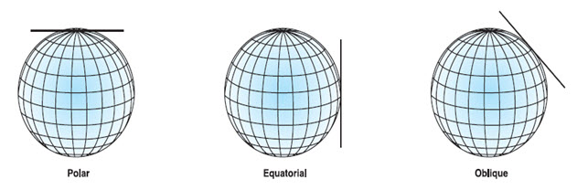
Fig. 23.8. Polar, Equatorial and oblique projections. (Source: Kennedy, 1994)

Polar aspects are the simplest form. Parallels of latitude are concentric circles centered on the pole, and meridians are straight lines that intersect at the pole with their true angles of orientation. In other aspects, planar projections will have graticular angles of 90 degrees at the focus. Directions from the focus are accurate. Great circles passing through the focus are represented by straight lines; thus the shortest distance from the center to any other point on the map is a straight line. Patterns of area and shape distortion are circular about the focus. For this reason, azimuthal projections accommodate circular regions better than rectangular regions. Planar projections are used most often to map polar regions. Some planar projections view surface data from a specific point in space. The point of view determines how the spherical data is projected onto the flat surface. The perspective from which all locations are viewed varies between the different azimuthal projections. Perspective points may be the center of the earth, a surface point directly opposite from the focus, or a point external to the globe, as if seen from a satellite or another planet.

Azimuthal projections are classified in part by the focus and, if applicable, by the perspective point.

The graphic below compares three planar projections with polar aspects but different perspectives. The Gnomonic projection views the surface data from the center of the earth, whereas the Stereographic projection views it from pole to pole. The Orthographic projection views the earth from an infinite point, as if viewed from deep space. Note how the differences in perspective determine the amount of distortion toward the equator. (ESRI Map projections.pdf)

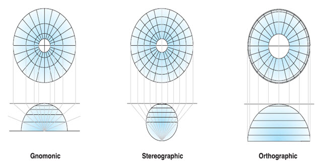
Fig. 23.9. Types of Azimuthal projection based on focus and perspective point.

(Source: Kennedy, 1994)

23.2 Projection Specification

A map projection by itself isn't enough to define a projected coordinate system. One can state that a dataset is in Transverse Mercator, but that's not enough information. Where is the center of the projection? Was a scale factor used? Without knowing the exact values for the projection parameters, the dataset can't be reprojected.

You can also get some idea of the amount of distortion the projection has added to the data. If you're interested in Australia but you know that a dataset's projection is centered at 0,0, the intersection of the equator and the Greenwich prime meridian, you might want to think about changing the center of the projection.

Each map projection has a set of parameters that you must define. The parameters specify the origin and customize a projection for your area of interest. (gistutorial.blogspot.com/2011/04/projection-parameters.html)

On the round surface of the earth, locations are described in terms of latitude and longitude. Some projection parameters, called angular parameters, are set with these latitude-longitude values. Once the earth's back has been broken with a projection, locations are described in terms of constant units like meters or feet. Some projection parameters, called linear parameters, use these constant units (or they use ratios, such as 0.5 or 0.9996).

(www.geo.hunter.cuny.edu/.../Projection%20parameters.htm).

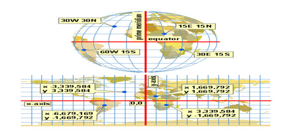
Fig. 23.10. Round data is described with meridians, parallels, and latitude-longitude values. Bottom: Flat data is described with x, y units. Projection parameters use both kinds of descriptions. The projection at bottom is Plate Carrée. (Source:www.geo.hunter.cuny.edu/.../Projection%20parameters.htm)

23.2.1 Angular parameters

(i)  Central meridian

Central meridian defines the origin of the x–coordinates. Every projection has a central meridian, which is the middle longitude of the projection. In most projections, it runs down the middle of the map and the map is symmetrical on either side of it. It may or may not be a line of true scale. (True scale means no distance distortion.)

In ArcGIS, you can change the central meridian of any projection. (Occasionally, it's the only angular parameter you can change.)The central meridian is also called the ‘longitude of origin’ or the ‘longitude of center’. Its intersection with the latitude of origin (see below) defines the starting point of the projected (x, y) map coordinates. (www.geo.hunter.cuny.edu/.../Projection%20parameters.htm).

(ii) Latitude of origin

Latitude of origin defines the origin of the y–coordinates. This parameter may not be located at the center of the projection. In particular, Conic projections use this parameter to set the origin of the y–coordinates below the area of interest. In that instance, you don't need to set a false northing parameter to ensure that all y–coordinates are positive.

(gistutorial.blogspot.com/2011/04/projection-parameters.html).

Every projection also has a latitude of origin. The intersection of this line with the central meridian is the starting point of the projected coordinates. In ArcGIS, you can put the latitude of origin wherever you want for most conic and transverse cylindrical projections. (In many world projections, on the other hand, it is defined to be the equator and can't be changed.) The latitude of origin may or may not be the middle latitude of the projection and may or may not be a line of true scale. The important thing to remember about the latitude and longitude of origin is that they don't affect the distortion pattern of the map. All they do is define where the map's x, y units will originate.

When data is unprojected, it doesn't have x, y units. Locations are measured in latitude and longitude, as you know from the previous module. But when you set a projection and flatten everything out, you also start using a new way to measure location. This new way is in terms of constant distance units (like meters or feet) measured along a horizontal x-axis and a vertical y-axis. A location like x = 500,000, y = 100,000 would refer to a point 500,000 meters (or whatever units of measure you are using) along the x-axis and 100,000 meters along the y-axis. The place where the axes cross is the coordinate origin, or 0,0 point. Commonly, this is in the middle of the map but it doesn't have to be.

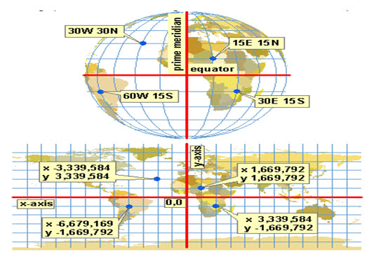
Fig. 23.11. In the top graphic below, the intersection of the central meridian (longitude of origin) and the latitude of origin is marked with a cross. This point becomes the origin of the x, y coordinates. The bottom graphic shows the grid (normally invisible) on which the x, y coordinates are located. The heavy lines are the x- and y-axes, which divide the grid into four quadrants. Coordinates are positive in one direction and negative in the other for each axis. (Source:www.geo.hunter.cuny.edu/.../Projection%20parameters.htm)

(iii) Standard parallel

A standard parallel is a line of latitude that has true scale. Not all projections have standard parallels, but many common ones do. Conic projections often have two. In a few projections, like the Sinusoidal and the Polyconic, every line of latitude has true scale and is therefore a standard parallel.

In ArcGIS, you can change the standard parallel for some projections and not for others. Many world projections, for instance, have fixed standard parallels.  A standard parallel may or may not coincide with the latitude of origin.

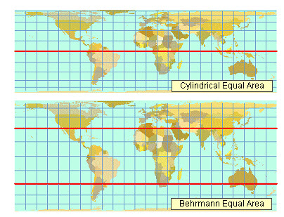
Fig. 23.12. Top: The Cylindrical Equal Area projection has a single standard parallel. By default, it is the equator, but you can change it. Bottom: The Behrmann projection is the same projection, but with two standard parallels at 30° N and 30° S. These standard parallels define the projection and cannot be changed. (Source:www.geo.hunter.cuny.edu/.../Projection%20parameters.htm)

(iv) Latitude of center

Latitude of center is used with the Hotine Oblique Mercator Center (both Two-Point and Azimuth) cases to define the origin of the y–coordinates. It is almost always the center of the projection (gistutorial.blogspot.com/2011/04/projection-parameters.html).

(v) Central parallel

Central parallel defines the origin of the y–coordinates.

NOTE:  In some projections, you will also see parameters called the latitude of center and the central parallel. These two terms seem to have the same meaning. Like the latitude of origin, they define the starting point of the y-coordinates; unlike it, they are nearly always the middle parallel of the projection. These parameters are used mainly with projections that have single points (rather than lines) of zero distortion, such as the Gnomonic and Orthographic. The intersection of the latitude of center (or central parallel) with the central meridian defines both the origin of the x, y coordinates and the point of zero distortion for the projection.

(www.geo.hunter.cuny.edu/.../Projection%20parameters.htm).

23.2.2 Linear parameters

(i) False easting and false northing

Linear parameters false easting is a linear value applied to the origin of the x coordinates. False northing is a linear value applied to the origin of the y coordinates. These are nothing but two big numbers that are added to each x- and y-coordinate, respectively. The numbers are big enough to ensure that all coordinate values or at least all those in your area of interest, come out positive. You can also use the false easting and northing parameters to reduce the range of the x or y coordinate values. For example, if you know all y values are greater than 5,000,000 meters, you could apply a false northing of -5,000,000. (gistutorial.blogspot.com/2011/04/projection-parameters.html).

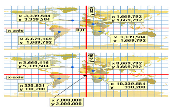
Fig. 23.13. Top: Projected coordinates are positive or negative, depending on their location. Bottom: A false easting value of 7,000,000 and a false northing value of 2,000,000 have been set. Every x-coordinate is now its original value plus 7,000,000. Every y-coordinate is its original value plus 2,000,000. The projection is Plate Carrée.

(Source:www.geo.hunter.cuny.edu/.../Projection%20parameters.htm)

(ii) Scale factor

A scale factor is the ratio of the true map scale to the stated map scale for a particular location. Scale factor is a unitless value applied to the centerpoint or line of a map projection. The scale factor is usually slightly less than one. The UTM coordinate system, which uses the Transverse Mercator projection, has a scale factor of 0.9996. Rather than 1.0, the scale along the central meridian of the projection is 0.9996. This creates two almost parallel lines approximately 180 kilometers, or about 1°, away where the scale is 1.0. The scale factor reduces the overall distortion of the projection in the area of interest. Learn more about the Transverse Mercator projection (gistutorial.blogspot.com/2011/04/projection-parameters.html). Remember that no map has true scale everywhere.

A line of true scale is defined as having a scale factor of 1.0. Along this line, the actual map scale is equal to the stated scale (there is no distortion of distance). A scale factor of 2.0 means that distance measurements on the map are twice too long—if your scale bar tells you it's a hundred kilometers from A to B, it's really only fifty kilometers. A scale factor of 0.5 means that distance measurements are twice too short. (www.geo.hunter.cuny.edu/.../Projection%20parameters.htm)

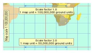
Fig. 23.14. A Mercator projection with a stated map scale of 1:100,000,000. Along a line of true scale, such as the equator in this projection, the scale factor is 1.0. One map unit equals the number of ground units that the map says it does. At 60° north or south, the scale factor increases to 2.0 along the parallels. The blue double-headed arrow at the bottom of the map measures only half as much ground as the one at the top.

(Source:www.geo.hunter.cuny.edu/.../Projection%20parameters.htm)

Table 23.1. Some examples of projected co-ordinate system (Source:www.geo.hunter.cuny.edu/.../Projection%20parameters.htm)

Projection	Central meridian (longitude)	Central parallel (latitude)	False easting	False northing	Scale factor
OS GB	20 W	490 N	+400 000	-100 000	0.999 601 2
UTM ϕ > 00	Zonal	00	+500 000	0	0.999 6
UTM ϕ < 00	Zonal	00	+500 000	-100 000	0.999 6
GK TM zone 11	630 E	00	+500 000	0	1

Keywords: Map projection, Cylindrical projection, Conic projection, Azimuthal projection, Angular parameter, Linear parameter

References

• Kennedy Melita, 1994, Understanding Map projections, Environmental Systems Research Institute, Inc., pp 15 -19.

• Class Notes Lecture, Map Projections.

• ESRI Map projections

• http://rnlnx635.er.usgs.gov/mac/isb/pubs/MapProjections/projections.html

• Laurie A. B. Garo, 1997, Introduction to Map Projections

• Arc GIS Online, 8/24/2012, ESRI Publication

• (egsc.usgs.gov/isb/pubs/factsheets/fs07701.html) The Universal Transverse Mercator (UTM) Grid, USGS, Fact Sheet 077-01 (August 2001)

• Projection parameter, GIS Tutorials (gistutorial.blogspot.com/2011/04/projection-parameters.html)

• Projection parameters (www.geo.hunter.cuny.edu/.../Projection%20parameters.htm)

Suggested Reading

• http://www.progonos.com/furuti/MapProj/Normal/ProjTbl/projTbl.html

• Rabu, 2009, GIS Tutorial, For College students Global Mapper  GIS