Remote Sensing & GIS Applications

Lesson 24 Map Algebra

24.1.1 Data types

This section focuses on map algebra operations available for gridded datasets, such as those implemented in ESRI's Spatial Analyst extension for ArcView. Similar operations are available in other grid-based GISes, such as GRASS (Geographic Resources Analysis Support System).

The data associated with any grid cell can be of any type whatsoever.  It is conceptually useful to divide data types into several classes, however.  These include:

• Categorical data: These are non-numerical data.  Grids that classify land use or land cover exemplify this category.  Other examples are proximity grids (values identify the nearest object) and feature grids (only two values are possible: one value for cells where features occur, another value--typically zero or NoData--where features do not occur).

• Integral data: These data may be relative ranks or preferences or they may be counts of occurrences or observations, for example. Thus, what they measure is inherently integral.

• Floating-point ("real" data).  These typically represent a real surface, such as elevation, or the values of a scalar function (a "conceptual surface," if you will).  Examples of such functions would be temperature, slope, amount of sunlight received per year, distance to the nearest feature, population density.

• Vector data: These are ordered tuples of real values that represent fields of directions.  For example, hydraulic gradients (for two-dimensional groundwater models), wind velocities (again for two-dimensional models), and ocean currents are two-dimensional vector fields.  Vector data may have more than two dimensions, even though they are defined over a strictly two-dimensional domain. For example, models using astronomical data, such as climate models, may make use of information about the three-dimensional location (on the earth's surface) of each grid point.

(Scientific visualization systems usually have built-in support for vector data, whereas most GISes require the modeler to represent vector data as an ordered collection of floating-point grids).

(http://www.quantdec.com/SYSEN597/GTKAV/section9/map_algebra.htm)

24.1.2 Working with null data

An essential part of map algebra or spatial analysis is the coding of data in such a way as to eliminate certain areas from further contribution to the analysis. For instance, if the existence of low-grade land is a prerequisite for a site selection procedure, we then need to produce a layer in which areas of low-grade land are coded distinctively so that all other areas can be removed. One possibility is to set the areas of low-grade land to a value of 1 and the remaining areas to 0. Any processes involving multiplication, division or geometric mean that encounter the zero value will then also return a zero value and that location (pixel) will be removed from the analysis. The opposite is true if processing involves addition, subtraction or arithmetic mean calculations, since the zero value will survive through to the end of the process. The second possibility is to use a null or No Data value instead of a zero. The null is a special value which indicates that there is no digital numerical value. In general, unlike zero, any expression will produce a null value if any of the corresponding input pixels have null values. Many functions and expressions simply ignore null values, however, and in some circumstances this may be useful, but it also means that a special kind of function must be used if we need to test for the presence of (or to assign) null values in a dataset. For instance, within ESRI’s ArcGIS, the function ISNULL is used to test for the existence of null values and will produce a value of 1 if null, or 0 if not. Using ER Mapper’s formula editor, null values can easily be assigned, set to other values, made visible or hidden. Situations where the presence of nulls is disadvantageous include instances where there are unknown gaps in the dataset, perhaps produced by measurement error or failure. Within map algebra, however, the null value can be used to great advantage since it enables the selective removal or retention of values and locations during analysis.

Table 24.1 Operations categorized according to their spatial or non-spatial nature.

Output	Spatial attributes involved?
	Yes	No (not necessarily)
Map or image	Neighbourhood processing(filtering), zonal and focal operations, mathematical morphology	Reclassification, rescaling (unary operations), overlay (binary operations), thresholding and density slicing.
Tabular	Spatial autocorrelation and variograms	Various tabular statistics (aggregation, variety) and tabular modeling (calculation of new fields from existing ones), scattergraphs

(Source: After Bonham-Carter, 2002)

24.1.3 Logical and conditional processing

These two processes are quite similar and they provide a means of controlling what happens during some function. They allow us to evaluate some criterion and to specify what happens next if the criterion is satisfied or not. Logical processing describes the tracking of true and false values through a procedure. Normally, in map algebra, a non-zero value is always considered to be a logical true, and zero, a logical false. Some operators and functions may return either logical true values (1) or logical false values (0), for example relational and Boolean operators. The return of a true or false value acts as a switch for one or other consequence within the procedure. Conditional processing allows that a particular action can be specified, according to the satisfaction of various conditions; if the conditions are evaluated as true then one action is taken, and an alternative action is taken when the conditions are evaluated as false. The conventional if–then–else statement is a simple example of a conditional statement:

if i < 16 then 1 else null where i = input pixel dn

Conditional processing is especially useful for creating analysis ‘masks’. In Fig. 24.1, each input pixel value is tested for the condition of having a slope equal to or less than 15º. If the value tests true (slope angle is 15º or less), a value of 1 is assigned to the output pixel. If it tests false (exceeds 15º), a null value is assigned to the output pixel. The output could then be used as a mask to exclude areas of steeper slopes and allow through all areas of gentle slopes, such as might be required in fulfilling the prescriptive criteria for a site selection exercise.

24.1.4 Other types of operator

Expressions can be evaluated using arithmetic operators (addition, subtraction, logarithmic, trigonometric) and performed on spatially coincident pixel DN values within two or more input layers (Table 24.2). Generally speaking, the order in which the input layers are listed denotes the precedence with which they are processed; the input or operator listed first is given top priority and is performed first, with decreasing priority from left to right.

A relational operator enables the construction of logical functions and tests by comparing two numbers and returning a true value (1) if the values are equal or false (0) if not. For example, this operator can be used to find locations within a single input layer with DN values representing a particular class of interest. These are particularly useful with discrete or categorical data.

A Boolean operator, for example AND, OR or NOT, also enables sequential logical functions and tests to be performed. Like relational operators, Boolean operators also return true (1) and false (0) values. They are performed on two or more input layers to select or remove values and locations from the analysis. For example, to satisfy criteria within a slope stability model, Boolean operators could be used to identify all locations where values in one input representing slope are greater than 40º AND where values in an elevation model layer are greater than 2000m (as in Fig. 24.2a).

Logical operators involve the logical comparison of the two inputs and assign a value according to the type of operator. For instance, for two inputs (A and B) A DIFF B assigns the value from A to the output pixel if the values are different or a zero if they are the same. An expression A OVER B assigns the value from A if a non-zero value exists; if not then the value from B is assigned to the output pixel. A combinatorial operator finds all the unique combinations of values among the attributes of multiple input rasters and assigns a unique value to each combination in the output layer. The output attribute will contain fields and attributes from all the input layers.

All these operators can be used, with care, alone or sequentially, to remove, test, process, retain or remove values (and locations) selectively from datasets alone or from within a spatial analysis procedure.

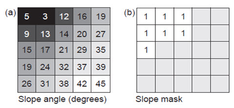
Fig. 24.1. Logical test of slope angle data, for the condition of being no greater in value than 15º: (a) slope angle raster and (b) slope mask (pale grey blank cells indicate null values). (Source: Liu, and Mason, 2009)

Table 24.2. Summary of common arithmetic, relational, Boolean, power, logical and combinatorial operator.

Arithmatic	Relational (return true/false)	Boolean (return true/false)
+, Addition -. Substraction *,Multiplication    /, Division            MOD, Modulus	= =. EQ Equal ^=,<>, NE Not equal <=.LT Less than/equal to <=LE Less than/equal to >,GT Greater than >=, GE greater than/ equal to	^,Not Logical complement                               & AND Logical AND                                       l, OR Logical OR                                                                  !, XOR Logical XOR
Power	Logical	Combianational
Sqrt, Square root Sqr, Square Pow, Raised to a power	DIFF, Logical difference IN{list}, Contained in list                                                     OVER, Replace	CAND, Combinational AND COR, Combinational OR CXOR, Combinational XOR

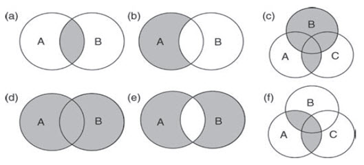
Fig. 24.2. Use of Boolean rules and set theory within map algebra; here the circles represent the feature classes A, B and C, illustrating how simple Boolean rules can be applied to geographic datasets, and especially rasters to extract or retain values, to satisfy a series of criteria: (a) A AND B (intersection or minimum ); (b) A NOT B; (c) (A AND C) OR B; (d) A OR B (union or maximum); (e) A XOR B; and (f) A AND (B OR C).

(Source: Liu, and Mason, 2009)

Table 24.3. Summary of local operations.

Type	Includes	Example
Primary	Creation of a layer from nothing	Rasters of constant value or containing randomly generated values
Unary	Conversion of units of measurement and as intermediary steps of spatial analysis	Rescaling, negation, comparing or applying mathematical functions reclassification
Binary	Operations on ordered pairs of numbers in matching pixels between layers	Arithmetic and logical combinations of rasters
N-ary	Comparison of local statistics between several rasters (many to one or many to many)	Change or variety detection

(Source: Liu  and Mason, 2009)

24.2 Local Operations

A local operation involves the production of an output value as a function of the value(s) at the corresponding locations in the input layer(s). These operations can be considered point operations when performed on ras­ter data, i.e. they operate on a pixel and its matching pixel position in other layers, as opposed to groups of neighbouring pixels. They can be grouped into those which derive statistics from multiple input layers (e.g. mean, median, minority), those which combine multiple input layers, those which identify values that satisfy specified criteria or the number of occurrences that satisfy specified criteria (e.g. greater than or less than), or those which identify the position in an input list that satisfies a specified criterion. All types of operator previously mentioned can be used in this context. Commonly they are subdivided according to the number of input layers involved at the start of the process. They include primary operations where nothing exists at the start, to n-ary operations where n layers may be involved; they are summarized in Table 24.3 and illustrated in Fig. 24.3.

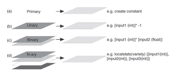
Fig. 24.3. Classifying map algebra operations in terms of the number of input layers and some examples.

(Source: Liu and Mason, 2009)

24.2.1 Primary operations

This description refers primarily to operations used to generate a layer, conceptually from nothing, for example the creation of a raster of constant value, or containing randomly generated numbers, such as could be used to test for error propagation through some analysis. An output pixel size, extent, data type and output DN value (either constant or ran­dom between set limits) must be specified for the creation of such a new layer.

24.2.2 Unary operations

These operations act on one layer to produce a new output layer and they include tasks such as rescaling, negation, comparison with other numbers, application of functions and reclassification. Rescaling is especially useful in preparation for multi-criteria analysis where all the input layers should have consistent units and value range: for instance, in converting from byte data, with 0 to 255 value range, to a percentage scale (0-100) or a range of between 0 and 1, and vice versa. Negation is used in a similar context, in modifying the value range of a dataset from being entirely positive to entirely nega­tive and vice versa. Comparisons create feature grids: the places where the comparison is true can be considered features on the earth's surface.  They map the regions where a logical condition (the comparison) holds.  These could be regions where, say, ozone concentrations exceed a threshold, ocean depths are below a certain target, or land use equals a given code. Mathematical functions are useful for changing the visualization of a grid.  An equal interval classification using the square roots of the values will differ from an equal interval classification of the values themselves, for instance.  Functions are also important as intermediate steps in many models. Reclassification is especially significant in data preparation for spatial analysis, and so deserves rather more in-depth description, but all these activities can be and are commonly carried out in image processing systems.

To illustrate different applications succinctly, suppose that three grids appear in the current view: "Integer" is an integer grid, "Float" is a floating-point grid, and "Indicator" is an integer grid containing only 0, 1, and NoData values.  A value of 0 can be interpreted as a logical "false" and a value of 1 as a logical "true".  In practice, of course, we will replace these names by the names of our themes.

• Rescale a grid: that is, Multiply all its values by a constant value.

[Float] * 3.1415927 Multiply all values by Pi

[Integer].Float * (39.37/12) Convert meters to feet

[Integer] * (-1) Negate all values

Not [Indicator] Negate all logical values: 0 becomes 1, 1 becomes 0

• Compare a grid to a constant value. The result of a comparison is true, 0 where the comparison is false, and NoData where the original value is NoData

[Float] < 1 Returns 1 where values are less than 1, otherwise returns 0

[Integer] = 0 Converts all zeros to ones and all other values to zeros

• Apply a mathematical (or logical) function to a grid, cell by cell.

[Float].Cos Computes the cosine of each value (interpreted as radians).

[Float].Int Rounds all values and converts the result to an integer grid.

[Float].Sqrt Computes the square root of each value.  Negative values return NoData (because the square root is not defined for negative values).

[Float].IsNull Returns 1 at all cells with NoData values, otherwise returns 0.

24.2.2.1 Reclassification

This involves the process of reassigning a value, a range of values, or a list of values in a raster to new output values, in a new output raster. If one class (or group or range of classes) is more interesting to us than the other classes, its original values can be assigned a specific value and all the others can be changed into a different (background) value. This involves the creation of a discrete raster from either a continuous one or another discrete raster. Reclassification can be applied to both vector and raster objects.

In the case of discrete raster data, a reclassification may be required to produce consistent units among a set of input raster images, in which case a one-to-one value change may be applied. The out­put raster would look no different, spatially, from the input, having the same number of classes, but the values would have changed.

Different classes or types of feature may be reclassified according to some criteria that are important to the overall analysis. During the reclassification process, weighting can be applied to the output values to give additional emphasis to the significant classes, and at the same time reduc­ing the significance of other classes.

The example in Fig. 24.4a shows a discrete raster representation of a geological map in which nine lithological units are coded with values 1 to 9 and labelled for the purposes of presentation, according to their name, rock type and ages. For the purposes of some analysis it may be neces­sary to simplify this lithological information, for example according to the broad ages of the units, PreCambrian, Palaeozoic and Mesozoic, for in­stance. The result of such a simplification is shown in Fig. 24.4c; now the map has only three classes and it can be seen that the older rocks (Precambrian and Palaeozoic) are clustered in the south-western part of the area, with the younger rocks (Mesozoic) forming the majority of the area as an envelope around the older rocks. So the simplification of the seemingly quite complex lithological information shown in Fig. 24.4a has revealed spatial patterns in that information which are of significance and which were not immediately apparent beforehand. Fig. 24.4d shows a second reclassification of the original lithological map, this time on the basis of relative permeability. The information is again simplified by reducing the number of classes to two, impermeable and permeable. Such a map might form a useful intermediary layer in an exer­cise to select land suitable for waste disposal but also illustrates that subjective judgements are in­volved at the early stage of data preparation. In the very act of simplifying information, we introduce bias and, strictly speaking, error into the analysis. We also have to accept the assumptions that the original classes are homogeneous and true represen­tations everywhere on the map, which they may not be. In reality there is almost certainly heterogeneity within classes and the boundaries between the clas­ses may not actually be as rigid as our classified map suggests.

Continuous raster data can also be reclassified in the same way. The image in Fig. 24.5a shows a DEM of the same area with values ranging between 37 and 277, representing elevation in meters above sea level. Reclassification of this dataset into three classes of equal interval to show areas of low, medium and high altitude produces the simplified image in Fig. 24.5b. Comparison with Fig. 24.5b shows that the areas of high elevation coincide with the areas where older rocks exist at the surface in the south-west of the area, again revealing spatial patterns not immediately evident in the original image. Reclassification of the DEM into three classes, this time with the classes defined according to the natural breaks in the image histo­gram (shown in Fig. 24.6), produces a slightly different result, Fig. 24.5c. The high-elevation areas are again in the south-west but the shape and distribution of those areas are different. This de­monstrates several things. Firstly, that very different results can be produced when we simplify data so that (and secondly) we should be careful in doing so, and, thirdly, that the use of the image histogram is fundamental to the understanding of and sensible use of reclassification of continuous raster data.

Reclassification forms a very basic but important part of spatial analysis, in the preparation of data layers for combination, in the simplification of layer information and especially when the layers have dissimilar value ranges. Reclassification is one of several methods of producing a common range among input data layers that hold values on different measurement scales.

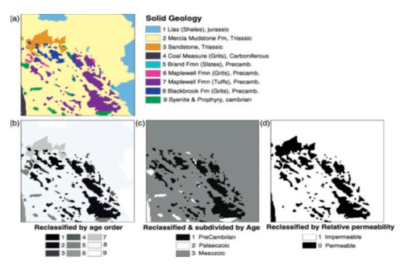
Fig. 24.4 (a) Discrete rastFig.er representation of a geological map, with nine classes representing different lithologies; (b) one-to-one reclassification by age order (1 representing the oldest, 9 the youngest); (c) a reclassified and simplified version where the lithological classes have been grouped and recoded into three broad age categories (Pre-Cambrian, Palaeozoic and Mesozoic); (d) a second reclassified version where the lithologies have been grouped according to their relative permeability, with 1 representing impermeable rocks and 0 permeable; such an image could be used as a mask. (Source: Liu and Mason, 2009)

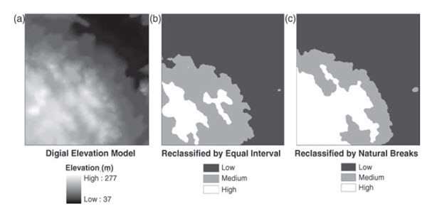
Fig. 24.5. (a) A DEM; (b) a DEM reclassified into three equal interval classes; and (c) a DEM reclassified into three classes by natural breaks in the histogram (shown in Fig. 24.6).

(Source: Liu and Mason, 2009)

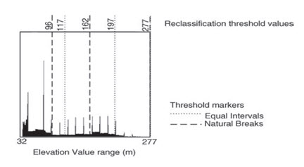
Fig. 24.6. Image histogram of the DEM shown in Fig. 24.5a and the positions of the reclassification thresholds set by equal interval and natural break methods (shown in Fig. 24.5b and c, respectively).

(Source: Liu and Mason, 2009)

24.2.3 Binary operations

Binary numeric operations act on ordered pairs of numbers.  Likewise, binary grid operations act on the pairs of numbers obtained in each set of matching cells.  The resulting grid is defined only where the two input grids overlap.

Suppose there are several floating-point grids represented by themes named "Float", "Float1", "Float2", and so on; with a similar supposition for integer and logical grids.

• Mathematical operators

[Float] + [Integer] Converts the values in [Integer] to floats, then performs the additions.

• Logical operators

[Float1] < [Float2]  Returns 1 in each cell where [Float1]'s value is less than [Float2]'s value; otherwise, returns 0.

(http://www.quantdec.com/SYSEN597/GTKAV/section9/map_algebra.htm)

[Indicator1] And [Indicator2] Returns 1 where both values are nonzero otherwise returns 0.

This description refers to operations in which there are two input layers, leading to the production of a single output layer. Overlay refers to the combi­nation of more than one layer of data, to create one new layer. The example shown in Fig. 24.7 illustrates how a layer representing average rainfall, and another representing soil type, can be combined to produce a simple, quali­tative map showing optimum growing conditions for a particular crop. Such operations are equiva­lent to the application of formulae to multiband images, to generate ratios, differences and other inter-band indices and as mentioned in relation to point operations on multi-spectral images, it is important to consider the value ranges of the input bands or layers, when combining their values arithmetically in some way. Just as image differencing requires some form of stretch applied to each input layer, to ensure that the real meaning of the differencing process is revealed in the output, here we should do the same. Either the inputs must be scaled to the same value range, or if the inputs represent values on an absolute measure­ment scale then those scales should have the same units.

The example shown in Fig. 24.7 represents two inputs with relative values on arbitrary nominal or ordinal (Fig. 24.7a) and interval (Fig. 24.7b) scales. The resultant values are also given on an interval scale and this is acceptable providing the range of potential output values is understood, having first understood the value ranges of the inputs, since they may mean nothing outside the scope of this simple exercise.

Another example could be the combination of two rasters as part of a cost-weighted analysis and possibly as part of a wider least cost pathway exercise. The two input rasters may represent mea­sures of cost, as produced through reclassification of, for instance, slope angle and land value, cost here being a measure of friction or the real cost of moving or operating across the area in question. These two cost rasters are then aggregated or summed to produce an output representing total cost for a particular area (Fig.24.8).

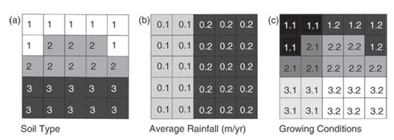
Fig. 24.7. An example of a simple overlay operation involving two input rasters: (a) an integer raster representing soil classes (class 2, representing sandy loam, is considered optimum); (b) a floating-point raster representing average rainfall, in metres per year (0.2 is considered optimum); and (c) the output raster derived by addition of a and b to produce a result representing conditions for a crop; a value of 2.2 (2 þ 0.2), on this rather arbitrary scale, represents optimum growing conditions and it can be seen that there are five pixel positions which satisfy this condition.

(Source: Liu and Mason, 2009)

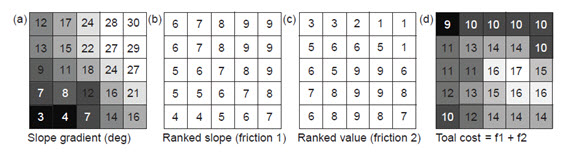
Fig. 24.8 (a) Slope gradient in degrees; (b) ranked (reclassified) slope gradient constituting  the first cost or friction input; (c) ranked land value (produced from a separate input land-use raster) representing the second cost or friction input; and (d) total cost raster produced by aggregation of the input friction rasters (f1 and f2). This total cost raster could then be used within a cost-weighted distance analysis exercise.

(Source: Liu and Mason, 2009)

24.2.4 N-ary operations

Here we deal with a potentially unlimited number of input layers to derive any of a series of standard statistical parameters, such as the mean, standard deviation, majority and variety. Ideally there should be a minimum of three layers involved but in many instances it is possible for the processes to be performed on single layers; the result may, however, be rather meaningless in that case. The more com­monly used statistical operations and their func­tionalities are summarized in Table 24.4. As with the other local operations, these statistical para­meters are point operations derived for each individual pixel position, from the values at correspond­ing pixel positions in all the layers, rather than from the values within each layer.

Table 24.4.  Summary of local pixel statistical operations, their functionality and input/output data format.

Statistic	Input format	Functionality	Data type
Variety         Mean	Only rasters. If a number is input, it will be converted to a raster constant for that value	Reports the number of different of different DN values occurring in the input rasters     Reports the average DN value among the input rasters	Output in integer         Output is floating point
Standard deviation	Rasters, numbers and constants	Reports the standard deviation of the DN values among the input rasters	Output is floating point
Medium             Sum   Range   Maximum   Minimum                 Minority	Only rasters. If a number is input, it will be converted to a raster constant for that value	Reports the middle DN value among the input raster pixel values. With an even number of inputs, the values are ranked and the middle two values are averaged. If inputs are all integer, output will be truncated to integer Reports the total DN value among the input rasters  Reports the difference between maximum and minimum DN Reports the highest DN value among the input rasters Reports the lowest DN value among the input rasters  Reports the DN value which occurs most frequently among the input rasters. If no clear majority, output = null, for example if there are three inputs all with different values. If all inputs have equal value, output=input  Reports the DN value which occurs least frequently among the input rasters. If no clear minority, as majority If only two inputs, where different, output= null. If all inputs equal, output = input. If only one input, output= input	If inputs are all integer, output will be integer, unless one is a float, there the input will be a float

(Source: Liu and Mason, 2009)

24.2.4.1 Local statistics

When we have many related grids defined in the same region, we often want to assess change: at each cell, how varied are the grid results?  How large do they get?  How small?  What is the average?  These questions make sense for numerical data.

For grids with ordinal data--that is, values that can be ordered, but which may not have any absolute meaning--you can still ask about order statistics.  These are the relative rankings of values within the ordered collections of values observed at each cell.

For grids with categorical data, you might want to know at each cell whether one category predominates throughout the collection of grids and how many different categories actually appear at the cell's location. (Liu, and Mason, 2009)

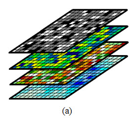
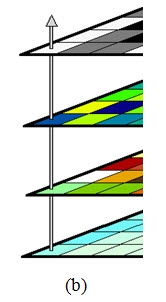
In all these cases, imagine a stack of grids with common mesh.

Fig. 24.9. (a) stack of grids with common mesh. (Source: http://www.quantdec.com/SYSEN597/GTKAV/section9/map_algebra.htm)

	At each cell location there is a stack of values, one for each grid. The N-ary operators create a new grid whose values depend on the stack of input data at each cell location.
Fig. 24.9. (b) New grid by N-ary operator. (Source: http://www.quantdec.com/SYSEN597/GTKAV/section9/map_algebra.htm)

The Spatial Analyst syntax for some of these requests is strange, because it wants to force expressions into the form "aGrid. Request (list of other grids)". This is inherently asymmetric because it singles out one grid in the collection to play the role of the object ("aGrid") to which the calculation is applied and leaves the other grids in the role of a list of arguments ("list of other grids").  Despite this syntax, for some requests, such as the local statistics, there is no asymmetry in the calculation itself: all the grids are equivalent.  For some other requests, there is an asymmetry in the calculation: one grid plays a special role.   

Spatial Analyst constructs lists with curly braces {} and separates the elements by commas.

• Compute local statistics

[Float]. LocalStats (#GRID_STATYPE_MAX, {[Float1], [Float2], [Float3]})  Computes the largest value among four grids.

[Float]. LocalStats (#GRID_STATYPE_MEDIAN, {[Float1], [Float2]})  Computes the median of three values.

[Integer]. LocalStats (#GRID_STATYPE_MAJORITY, {[Integer1], [Integer2]})  Computes the value occurring the most times (out of the three input values at each cell).  If two or more values occur an equal number of times, Spatial Analyst returns NoData.

The Majority statistic evidently is not very useful when many ties occur: that is, when there are many cells where two or more values occur equally often.

(http://www.quantdec.com/SYSEN597/GTKAV/section9/map_algebra.htm)

• Compare one grid (a “base’ grid) to many others simultaneously

[Float]. Grids Greater than ({[Float1], [Float2], [Float3], [Float4]}) For each base cell in [Float], computes the number of times corresponding cells from [Float1], ..., [Float4] exceed (and do not equal) the base cell’s value. There is a corresponding Grids Less Than operator.

• Combine the values of two grids based on values at a third grid

[Indicator]. Con ([Float1], [Float2]) Creates a grid with the values of [Float1] where [Indicator] is nonzero and with the values of [Float2] where [Indicator] is zero.

The Con request is especially useful. The result of Con, by default, is the second grid ([Float2] or [Mosaic] in the examples).  However, at cells where [Indicator] is true, the values of the first grid ([Float1] or [Average]) are "painted" over the default values.  Thus the Con request is a natural vehicle for selectively editing grids.                                                                                    

(http://www.quantdec.com/SYSEN597/GTKAV/section9/map_algebra.htm)

Keywords: Map algebra, proximity grids, null data, Local operations, Primary operations, Unary operations, Reclassification, Binary operations Mathematical operators, Logical operators, N-ary operations, Local statistics

References

• Jian Guo Liu, Philippa J. Mason, “Essential Image Processing and GIS for Remote Sensing,” Imperial College London, UK, 261-280 (2009).

• 1997. User Interfaces for Map Algebra. Journal of the Urban and Regional Information Systems Association, Vol.9, No. 1, pp. 44-54.

• http://www.quantdec.com/SYSEN597/GTKAV/section9/map_algebra2.htm