Site pages
Current course
Participants
General
MODULE 1. Fundamentals of Soil Mechanics
MODULE 2. Stress and Strength
MODULE 3. Compaction, Seepage and Consolidation of...
MODULE 4. Earth pressure, Slope Stability and Soil...
Keywords
29 March - 4 April
5 April - 11 April
12 April - 18 April
19 April - 25 April
26 April - 2 May
LESSON 13. Stress Path
13.1. What is Stress path?
Stress path is used to represent the successive states of stress in a test specimen of soil during loading or unloading. Series of Mohr circles can be drawn to represent the successive states of stress, but it is difficult to represent number of circles in one diagram. Figure 13.1 shows number of Mohr circles by keeping σ3 and increasing σ1 on σ - t plane. The successive states of stress can be represented by a series of stress points and a locus of these points (in the form of straight or curve) is obtained. The locus is called stress path. The stress points on σ - t plane can be transferred to p-q plane (as shown in Figure 13.1). The coordinates of the stress points on p-q plane can be obtained as:
\[p={{{\sigma _v} + {\sigma _h}} \over 2}\] (13.1)
\[q={{{\sigma _v} - {\sigma _h}} \over 2}\] (13.2)
The stress path can be drawn as:
(a) Total stress path (TSP)
(b) Effective stress path (ESP)
(c) Stress path of total stress minus static pore water pressure (TSSP)
If in a field situation, static ground water table exists, initial pore water pressure u0 will act on the sample. Thus, the static pore water pressure will be equal to u0. The effective stress coordinates of the stress points on p'-q' plane can be obtained as:
\[p'={{{\sigma _v} - u + {\sigma _h} - u} \over 2} = {{{{\sigma '}_v} + {{\sigma '}_h}} \over 2}\] (13.3)
\[q'={{{\sigma _v} - u - ({\sigma _h} - u)} \over 2} = {{{{\sigma '}_v} - {{\sigma '}_h}} \over 2} = {{{\sigma _v} - {\sigma _h}} \over 2}=q\] (13.4)
Figure 13.2 shows different stress paths for normally consolidated clay obtained from CU (effective) test.
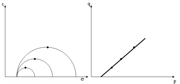
Fig. 13.1. Stress point on Mohr circle and on p-q plane.
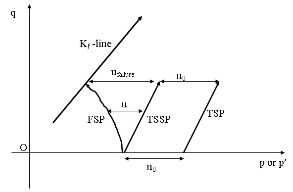
Fig.13.2. Different stress paths.
For initial condition, σv =σh =0 and if σv and σh are increased in such as way that ratio σh /σv is constant. This ratio is called lateral stress ratio, K. Thus,
\[K={{{\sigma _h}} \over {{\sigma _v}}}\] (13.5)
Similarly, coefficient of lateral earth pressure at rest (K0) and at failure (Kf) can be expressed as:
\[{K_0}={{{{\sigma '}_h}} \over {{{\sigma '}_v}}}\] (13.6)
\[{K_f}={{{{\sigma '}_{hf}}} \over {{{\sigma '}_{vf}}}}\] (13.7)
On p-q plane, the stress ratios are representing straight lines (as shown in Fig. 13.3).
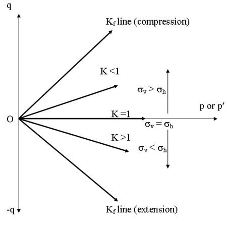
Fig. 13.3. Variation of Stress Rations.
Figure 13.4 shows the relationship between Kf line (on p-q plane) and Mohr-Colomb failure envelope (on s - t plane). The shear strength parameters can also be determined from Kf line on p-q plane as:
\[\phi={\sin ^{ - 1}}(\tan \psi )\] (13.8)
\[c={a \over {\cos \phi }}\] (13.9)
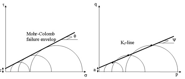
Fig. 13.4. Relationship between Kf line and Mohr-Colomb failure envelope.
References
Ranjan, G. and Rao, A.S.R. (2000). Basic and Applied Soil Mechanics. New Age International Publisher, New Delhi, India
PPT of Professor N. Sivakugan, JCU, Australia.
Suggested Readings
Ranjan, G. and Rao, A.S.R. (2000) Basic and Applied Soil Mechanics. New Age International Publisher, New Delhi, India.
Arora, K.R. (2003) Soil Mechanics and Foundation Engineering. Standard Publishers Distributors, New Delhi, India.
Murthy V.N.S (1996) A Text Book of Soil Mechanics and Foundation Engineering, UBS Publishers’ Distributors Ltd. New Delhi, India.
Last modified: Monday, 23 September 2013, 9:28 AM