Strength of Material

LESSON 23. Columns and Struts

\[{P_E} = {{{\pi ^2}E{I_{\min }}} \over {l_{eff}^2}}\]                                                   (23.2)

\[\Rightarrow {P_E} = {{{\pi ^2}AE} \over {l_{eff}^2}}{{{I_{\min }}} \over A} = {{{\pi ^2}AE} \over {l_{eff}^2}}k_{\min }^2\]  [ \[{k_{\min }} = \sqrt {{{{I_{\min }}} \over A}} \] is minimum the radius of gyration ]

\[\Rightarrow {{{P_E}} \over A} = {\pi ^2}E{\left( {{{{k_{\min }}} \over {{l_{eff}}}}} \right)^2}\]                              (23.3)

Now \[{{P_E}} /{E \le {\sigma _c}}\] , where, σ_c is the crushing stress of a short column. Therefore,

\[{\pi ^2}E{\left( {{{{k_{\min }}} \over {{l_{eff}}}}} \right)^2} \le {\sigma _c}\]

\[\Rightarrow {{{l_{eff}}} \over {{k_{\min }}}} \ge \sqrt {{{{\pi ^2}E} \over {{\sigma _c}}}}\]

Therefore the Euler buckling theory is applicable only when the slenderness ratio \[{{{l_{eff}}} /{{k_{\min }}} \]  has a minimum value. For instance, mild steel has the following properties,

E = 208GPa

σ_c = 320MPa

\[{{{l_{eff}}} \over {{k_{\min }}}}=\ge \sqrt {{{{\pi ^2}208 \times {{10}^9}} \over {320 \times {{10}^6}}}}=80\]

Therefore, for mild steel column if the slenderness is greater than 80, then only the Euler theory can be applied in order to predict the buckling load.

Moreover, in Euler’s theory it was assumed that the member is perfectly straight and homogeneous. Moreover the line of action of the applied load is assumed to be coincident with the centroidal axis of the column and therefore does not produce any moment. However in practical situations, column which satisfies all these idealization does not exist. This imposes further limitation on the direct application of Euler model in practical columns. In this lesson we will study the behavior of imperfect column and compare it with the Euler model derived in the last lesson.

23.2 Eccentrically Loaded Columns – Secant Formula

Consider an eccentrically loaded slender column as shown in Figure 23.1a.

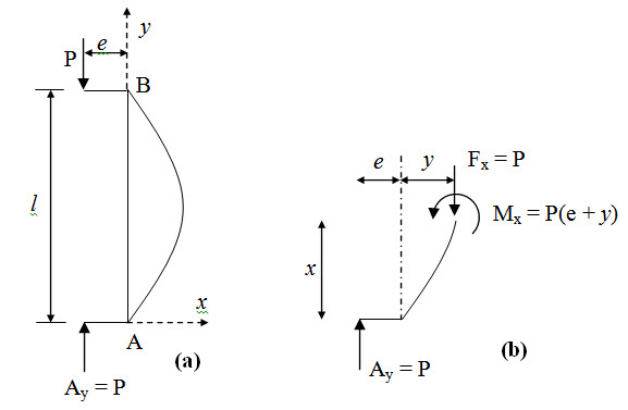
Fig. 23.1.

The equation of elastic line becomes,

\[{{{d^2}y} \over {d{x^2}}}=-{{{M_x}} \over {EI}}\]                                     (23.1)

\[\Rightarrow {{{d^2}y} \over {d{x^2}}} + {P \over {EI}}\left( {e + y} \right) = 0\]     (23.2)

\[\Rightarrow {{{d^2}y} \over {d{x^2}}} + {k^2}y=-{k^2}e\]                                          (23.3)

where, \[{k^2} = {P / {EI}}\]

The general solution of equation (23.3) is,

\[y=A\cos kx + B\sin kx - e\]                           (23.4)

Constants A and B are determined from the boundary conditions as follows,

\[y(x = 0)=0 \Rightarrow A=e\]

\[y(x = l)=0 \Rightarrow B={{1 - \cos kl} \over {\sin kl}}e\]

Substituting A and B in equation (23.4) yields,

\[y=\left( {\cos kx + {{1 - \cos kl} \over {\sin kl}}\sin kx - 1} \right)e\]                               (23.5)

Lateral deflection at mid-height (y = l/2),

\[{\left. y \right|_{x = l/2}}=\left( {\cos {{kl} \over 2} + {{1 - \cos kl} \over {\sin kl}}\sin {{kl} \over 2} - 1} \right)e\]                          (23.6)

\[\Rightarrow {\left. y \right|_{x = l/2}}=\left( {\sec {{kl} \over 2} - 1} \right)e\]                                                (23.7)

Writing equation (23.7) in terms of Euler load \[{P_E}={\pi ^2}EI/{l^2}\]  ,

\[{\left. y \right|_{x = l/2}}=\left[ {\sec \left( {{\pi\over 2}\sqrt {{P \over{{P_E}}}} } \right) - 1} \right]e\]                                    (23.8)

 

 

Suggested Readings

Yoo, C.H., Lee, S.C. (2011). Stability of Structures: Principles and Applications. Elsevier. 

Gere, J.M, Timoshenko S.P. (2010). Theory of Elastic Stability. Second Edition, Tata McGraw - Hill Education.