Watershed Hydrology

Lesson 29 Hydrologic Reservoir Routing

 29.1.1Reservoir Routing

In Reservoir routing the effect of a flood wave entering a reservoir is studied. Knowing the volume-elevation characteristic of the reservoir and the outflow-elevation relationship for the spillways and other outlet structures in the reservoir, the effect of a flood wave entering the reservoir is studied to predict the variations of reservoir elevation and outflow discharge with time. This form of reservoir routing is essential (i) in the design of the capacity of spillways and other reservoir outlet structures, and (ii) in the location and sizing of the capacity of reservoirs to meet specific requirements. 

29.1.2Channel Routing

In Channel routing the change in the shape of a hydrograph as it travels down a channel is studied. By considering a channel reach and an input hydrograph at the upstream end, this form of routing aims to predict the flood hydrograph at various sections of the reach. Information on the flood-peak attenuation and the duration of high-water levels obtained by channel routing is of utmost importance in flood-forecasting operations and flood-protection works. 

 

29.2 Uses of Flood Routing

The hydrologic analysis of problems such as flood forecasting, flood protection, reservoir design and spillway design invariably include flood routing.

 

29.3 Methods of Flood Routing

A variety of routing methods are available and they can be broadly classified into two categories as: (i) hydrologic routing, and (ii) hydraulic routing.

Hydrologic-routing methods employ essentially the equation of continuity. 

Hydraulic methods, on the other hand, employ the continuity equation together with the equation of motion of unsteady flow. The basic differential equations used in the hydraulic routing, known as St. Venant equations afford a better description of unsteady flow than hydrologic methods.

 

29.4 Basic Equations

The passage of a flood hydrograph through a reservoir or a channel reach is an unsteady-flow phenomenon. It is classified in open-channel hydraulics as gradually varied unsteady flow. The equation of continuity used in all hydrologic routing as the primary equation states that the difference between the inflow and outflow rate is equal to the rate of change of storage, i.e.

 (29.1)

 

WhereI is inflow rate, Q is outflow rate and S= storage

 

Alternatively, in a small time interval Δt the difference between the total inflow volume and total outflow volume in a reach is equal to the change in storage in that reach

 (29.2)

Where  is average inflow in time Δt,  is average outflow in time Δt, and  change in storage.

 

By taking  ,  and  ΔS = S₂ - S₁  with suffixes 1 and 2 to denote the beginning and end of time interval Δt, Eq. 29.2 is written as

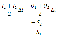 (29.3)

 

The time interval Δt should be sufficiently short so that the inflow and outflow hydrographs can be assumed to be straight lines in that time interval. Further Δt must be shorter than the time of transit of the flood wave through the reach.

 

In the differential form the equation or continuity for unsteady now in a reach with no lateral flow is given by

 (29.4)

Where T is top width of section, y isdepth of flow

 

The equation of motion for a flood wave is derived from the application of the momentum equation as

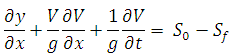 (29.5)

WhereV is velocity of flow at any section, S₀is channel bed slope;S_f is slope of the energy line.

 

Equation 29.4 and 29.5 are commonly known as St. Venant equations

  (29.3)

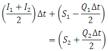
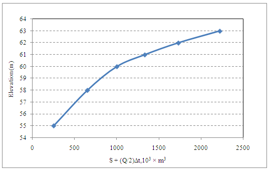
29.5 Hydrologic Reservoir Routing using Modified Pul’s Method

Equation 29.3 is rearranged as

At the starting of flood routing, the initial storage and outflow discharges are known.

This method requires construction of only two curves (i) S curve and (ii)    curve.

 

Following steps are followed to compute reservoir hydrologic routing using Modified Pul’s method.

1. From the inflow hydrograph, obtain the volume of water entering the reservoir in the short time interval, i.e., Compute average inflow  .
2. For an initial outflow obtain  from S curve and compute  .
3. Add average inflow   and   to obtain  .
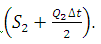4. Using computed values  , obtain Q₂ from the   curve.
5. Repeat the entire procedure to complete the routing.

 

Example 1

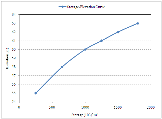
A small reservoir has the following storage elevation relationship

Elevation (m)	55.00	58.00	60.00	61.00	62.00	63.00
Storage (103  m3)	250	650	1000	1250	1500	1800

 

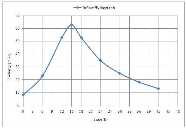
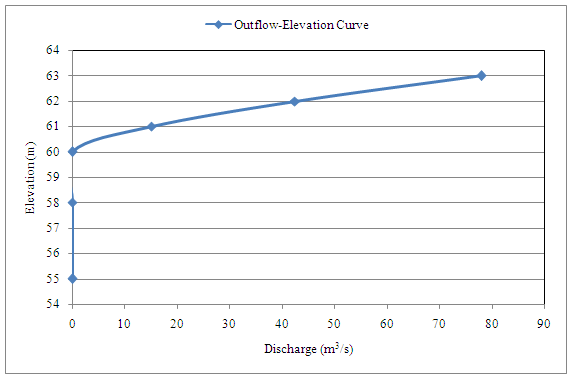
A spillway provided with its crest at elevation 60.00 m has the discharge relationship. Q = 15H^3/2, where H = head of water over the spillway crest.When the reservoir elevation is at 58.00 m a flood as given below enters the reservoir.

 

Route the flood and determine the maximum reservoir elevation, peak outflow and attenuation of the flood peak using Modified Pul’s method.

 

Time (h)	0	6	12	15	18	24	30	36	42
Inflow (m3/s)	8	23	53	63	53	35	25	18	13

 

Answer

 

 

Routing period	I1(m3/s)	I2(m3/s)		Q1(m3/s)			Q2(m3/s)	Elevation at beginning (m)	Elevation at end (m)
0-3	8	14.5	121.5	0	650	771.5	0	58	58.6
3-6	14.5	23	202.5	0	771.5	974	0	58.6	59.8
6-9	23	38.5	332.1	0	974	1306.1	13	59.8	60.8
9-12	38.5	53	494.1	13	1165.7	1659.8	39	60.8	61.9
12-15	53	63	626.4	39	1238.6	1865	52.5	61.9	62.4
15-18	63	53	626.4	52.5	1298	1924.4	57	62.4	62.5
18-21	53	43	518.4	57	1308.8	1827.2	50.5	62.5	62.3
21-24	43	35	421.2	50.5	1281.8	1703	42	62.3	62
24-27	35	29	345.6	42	1249.4	1595	35	62	61.8
27-30	29	25	291.6	35	1217	1508.6	29	61.8	61.6
30-33	25	22	253.8	29	1195.4	1449.2	24	61.6	61.4
33-36	22	18	216	24	1190	1406	20.5	61.4	61.2
36-39	18	15	178.2	20.5	1184.6	1362.8	17	61.2	61.05
39-42	15	13	151.2	17	1179.2	1330.4	14	61.05	60.9

 

 

References

Subramanya, K.(2008). Engineering Hydrology.Third edition, Tata McGraw Hill, 280-290.

 

Suggested Reading

Singh, V. P. (1994). Elementary Hydrology.Prentice Hall of India Private Limited, New Delhi.