Watershed Hydrology

Lesson 30 Hydrologic Channel Routing

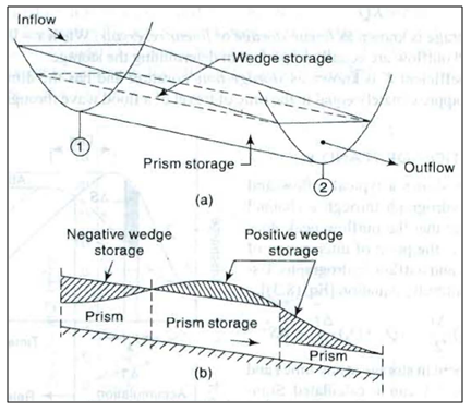
Fig. 30.1.Storage in Channel Reach. (Source: Subramanya, 2008)

30.1.1Prism Storage

It is the volume that would exist if the uniform flow occurred at the downstream depth, i.e. the volume formed by an imaginary plane parallel to the channel bottom drawn at the outflow section water surface.

 

30.1.2Wedge Storage

It is the wedge-like volume formed between the actual water surface profile and the top surface of the prism storage.

 

At a fixed depth at a downstream section of a river reach, the prism storage is constant while the wedge storage changes from a positive value at an advancing flood to a negative value during a receding flood.

 

The prism storage S_pis similar to a reservoir and can be expressed as a function of the outflow discharge, S_p =f (Q). The wedge storage can be accounted for by expressing it as S_w=f (I). The total storage in the channel reach can then be expressed as

 (30.1)

WhereK and x are coefficients and m is a constant exponent. It has been found that the value of m varies from 0.6 for rectangular channels to a value of about 1.0 for natural channels.

  

Muskingum Equation

Using m = 1.0, Eq. (30.1) reduces to a linear relationship for S in terms of I and Q as

 (30.2)

And this relationship is known as the Muskingum equation. In this the parameter x is known as weighting factor and takes a value between 0 and 0.5. When x = 0, the storage is a function of discharge only and Eq. (30.2) reduces to

 (30.3)

Such storage is known as linear storage or linear reservoir.

The coefficient K is known as storage-time constant and has the dimensions of time. It is approximately equal to the time of travel of a flood wave through the channel reach.

 

Estimation of K and x

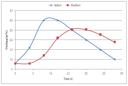
Figure 30.2 shows a typical inflow and outflow hydrograph through a channel reach.

 

Using the continuity equation,  the increment in storage at any time t and time element Δtcan be calculated. Summation of the various incremental storage values enable to find the channel storage Svstimet relationship (Fig. 30.2)

 

If an inflow and outflow hydrograph set isavailable for a given reach, values of S at various time intervals can be determined by the above technique. By ­choosing a trial value of x, values of S at any time tare plotted against the corresponding  values. If the value of x is chosen correctly, a straight-line relationship will result. However, if an incorrect value of x is used, the plotted points will trace a looping curve. By trial and error a value of x is so chosen that the data very nearly describe a straight line. The inverse slope of this straight line will give the value of K. Normally, for natural channels, the value of x lies between 0to 0.3. For a given reach, the values of x and K are assumed to be constant.

Fig. 30.2.Hydrographs and Storage in Channel Routing.

(Source: Subramanya, 2008)

30.2 Muskingum Method of Flood Routing

For a given channel reach by selecting a routing interval Δt and using the Muskingum equation, the change in storage is

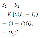 (30.4)

where suffixes 1 and 2 refer to the conditions before and after the time interval Δt. The continuity equation for the reach is

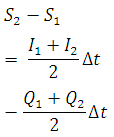 (30.5)

From Eqs (30.4) and (30.5),  is evaluated as

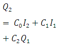 (30.6)

where

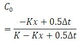 (30.6a)

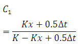 (30.6b)

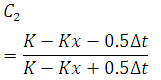 (30.6C)

Note that C0 + C1 + C2 = 1.0, Eq. 30.6 can be written in a general form for the n^th time step as

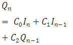 (30.6A)

Equation (30.6)isknown as Muskingum Routing Equation and provides a simple linear equation for channel routing. It has been found that for best results the routing interval Δt should be so chosen that K>Δt> 2Kx.

 

To use the Muskingum equation to route a given inflow hydrograph througha reach, the values of K and x for the reach and the value of the outflow, Q₁, from the reach at the start are needed. The procedure is described as follows

1. Knowing K and x, select an appropriate value of Δt.
2. Calculate C₀, C₁ and C₂.
3. Starting from the initial conditions I₁, Q₁ and known I₂at the end of the first time step Δt calculate Q₂by Eq. (30.6).
4. The outflow calculated in step (c) becomes the known initial outflow for the next lime step. Repeat the calculations for the entire inflow hydrograph.

 Example 1

Route the following flood hydrograph through a river reach for which Muskingum coefficient K = 8 h and x = 0.25.

Time (h)	0	4	8	12	16	20	24	28
Inflow (m3/s)	8	16	30	30	25	20	15	10

 

The initial outflow discharge from the reach is 8.0m³/s

 

Answer

Given: K =  8 h; x =  0.25; Δt = 4  

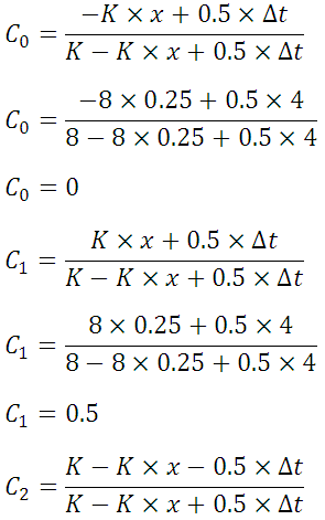
C₂ = 0.5

C₀ + C₁ + C₂ = 1.0

0 + 0.5 + 0.5 = 1.0

For the first time interval, 0 to 4 h,

I₁ = 8.0                    C₁I₁ = 4

I₂ = 16.0                  C₀I₂ = 0

Q₁ = 10.0                C₂Q₁ = 4 

Q₂ = C₀I₂ + C₁L₁ + C₂Q₁

Q₂ = 0 + 4 + 4 = 8

For the next time step, 4 to 8 h, Q₁ = 8.0  m³ / s

Muskingum channel routing results for further time steps are given in following

 

Table

Time (h)	Inflow	0 ×I2	0.5 ×I1	0.5 ×Q1
0	8				8
		0	4	4
4	16				8
		0	8	4
8	30				12
		0	15	6
12	30				21
		0	15	10.5
16	25				25.5
		0	12.5	12.75
20	20				25.25
		0	10	12.625
24	15				22.625
		0	7.5	11.3125
28	10				18.8125

 

 

References

Subramanya, K. (2008). EngineeringHydrology, Third edition, Tata McGraw Hill, 291-296.

 

Suggested Reading

Singh, V. P. (1994). Elementary Hydrology.Prentice Hall of India Private Limited,New Delhi.