System Engineering

LESSON 1. TRANSPORTATION PROBLEMS

 1. Introduction

Industries  require to transport their products available at several sources or production centres to a number of destinations or markets. In the process of distributing to various destinations, high transportation costs are involved. Minimizing the transportation cost will benefit the organisation by increasing the profit. To analyze and minimize the cost of transportation, transportation model is used.  The name “transportation model” is, however, misleading. This model can be used for a wide variety of situations such as scheduling, personnel assignment, product mix problems and many others, so that the model is really not confined to transportation or distribution only.

The origin of transportation models dates back to 1941 when F.L. Hitchcock presented a study entitled ‘The Distribution of a Product from Several Sources to Numerous Localities’. The presentation is regarded as the first important contribution to the solution of transportation problems. In 1947, T.C. Koopmans presented a study called ‘Optimum Utilization of the Transportation System’. These two contributions are mainly responsible for the development of transportation models which involve a number of production centres / sources and a number of destinations / markets. Each shipping source has a certain capacity and each destination has a certain requirement associated with a certain cost of transportation from the sources to the destinations. The objective is to minimize the cost of transportation while meeting the requirements at the destinations. Transportation problems may also involve movement of a product from plants to warehouses, warehouses to wholesalers, wholesalers to retailers, retailers to customers, etc.

 2. Assumptions in the Transportation Model

1. Total quantity of the items available at different sources/ supply is equal to the total requirement/ demand at different destinations / markets.

2. Items can be transported conveniently from all sources to destinations.

3. The unit transportation cost of the item from all sources to destinations is known.

4. The transportation cost on a given route is directly proportional to the number of units shipped on that route.

5. The objective is to minimize the total transportation cost for the organization as a whole and not for individual supply and distribution centres.

3. Definition of the Transportation Model

Suppose that there are m sources and n destinations. Let a_i be the number of supply units available at source i(i = 1,2,3,….., m) and let b_j be the number of demand units required at destination j(j = 1,2,3,….., n). Let c_ij represent the unit transportation cost for transporting the units from source i to destination j. The objective is to determine the number of units to be transported from source i to destination j so that the total transportation cost is minimum. In addition, the supply limits at the sources and the demand requirements at the destinations must be satisfied exactly.

If x_ij (x_ij ≥ 0) is the number of units shipped from source i to destination j, then the equivalent linear programming model will be

 Find x_ij (i =1,2,3, ……… , m ;  j = 1,2,3,……… , n) in order to

minimize     

                     _{m   n}                 

             z =   Σ    Σ   c_ij x_ij ,

                    ^{i =1    j = 1}    

subject to

          _n                   

              Σ   x_ij  = a_i ,   i = 1,2,3, …….. , m ,

 ^{j = 1}    

 and

               _m                

              Σ  x _ij  = b_j ,   j = 1,2,3, …….. , n ,

             ^{i= 1}

where    x _ij ≥ 0

The two sets of constraints will be consistent i.e., the system will be in balance if

                     _{m               n}                     

                    Σ  a_i  =     Σ  b_j   .

       ^{i =1            j = 1}    

Equality sign of the constraints causes one of the constraints to be redundant (and hence it can be deleted) so that the problem will have (m + n - 1) constraints and (m x n ) unknowns.

 Note that a transportation problem will have a feasible solution only if the above restriction is satisfied. Thus,

                     _{m               n}                     

                    Σ  a_i  =    Σ  b_j   is necessary as well as a sufficient condition for a

       ^{i =1          j = 1}    

transportation problem to have a feasible solution. Problems that satisfy this condition are called balanced transportation problems. Techniques have been developed for solving balanced or standard transportation problems only. It follows that any non – standard problem in which the supplies and demands do not balance, must be converted to a standard transportation problem before it can be solved. This conversion can be achieved by the use of a dummy source/destination.

The above information can be put in the form of a general matrix shown below:

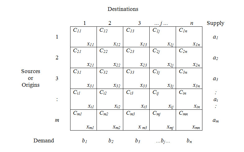
In table , c_ij  , i = 1,2, ….., m ;  j = 1,2, …… , n , is the unit shipping cost from the ith oringin to jth destination, x_ij is the quantity shipped from the ith origin to jth destination, a_i  is the supply available at origin i and b_j is the demand at destination j.

 Definitions:

 A few terms used in connection with transportation models are defined below.

1.  Feasible solution: A feasible solution to a transportation problem is a set of non-negative allocations, x_ij that satisfies the rim (row and column) restrictions.

2.  Basic feasible solution: A feasible solution to a transportation problem is said to be a basic feasible solution if it contains no more than m + n – 1 non – negative allocations, where m is the number of rows and n is the number of columns of the transportation problem.

3. Optimal solution: A feasible solution (not necessarily basic) that minimizes (maximizes) the transportation cost (profit) is called an optimal solution.

4.  Non -degenerate basic feasible solution: A basic feasible solution to a (m x n) transportation problem is said to be non – degenerate if,

1.  the total number of non-negative allocations is exactly m + n – 1 (i.e., number of independent constraint equations), and
2. these m + n – 1 allocations are in independent positions.
5. Degenerate basic feasible solution: A basic feasible solution in which the total number of non-negative allocations is less than m + n – 1 is called degenerate basic feasible solution.

4. Matrix Terminology

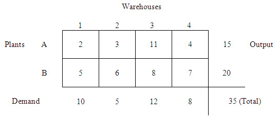
 The matrix used in the transportation models consists of squares called ‘cells’, which when stacked form ‘columns’ vertically and ‘rows’ horizontally.

 The cell located at the intersection of a row and column is designated by its row and column headings. Thus the cell located at the intersection of row A and column 3 is called cell (A, 3). Unit costs are placed in each cell.

  

5. Degeneracy in Transportation Problem

In case of simplex algorithm, the basic feasible solution may become degenerate at the initial stage or at some intermediate stage of computation. In a transportation problem with m origins and n destinations if a basic feasible solution has less than m + n – 1 allocations (occupied cells), the problem is said to be a degenerate transportation problem.

While in the simplex method degeneracy does not cause any serious difficulty, it can cause computational problem in transportation technique. In stepping – stone method it will not be possible to make close paths (loops) for each and every vacant cell and hence evaluations of all the vacant cells cannot be calculated. If modified distribution method is applied, it will not be possible to find all the dual variables u_i and v_j since the number of allocated cells and their c_ij values is not enough. It is thus necessary to identify a degenerate transportation problem and take appropriate steps to avoid computational difficulty. Degeneracy can occur in the initial solution or during some subsequent iteration.

 5.1. Degeneracy in the initial solution

Normally, while finding the initial solution (by any of the methods), any allocation made either satisfies supply or demand, but not both. If, however, both supply and demand are satisfied simultaneously, a row as well as column are cancelled simultaneously and the number of allocations become two less than m + n – 1 and so on.  This degeneracy is resolved or the above degenerate solution is made non-degenerate in the following manner:

First of all the requisite number of vacant cells with least unit costs are chosen so that (incase of tie choose arbitrarily):

1. these cells plus the existing number of allocations are equal to m + n – 1.

2. these  m + n – 1 cells are in independent positions i.e., no closed path (loop) can be formed among them. If a loop is formed the cells / cells with next lower cost is/are chosen so that no loop is formed among them. This can always be done if the solution we start with contains allocated cells in independent positions.

Now allocate an infinitesimally small but positive value ε (Greek letter epsilon) to each of the chosen cells. Subscripts are used when more than one such letter is required (e.g., ε1, ε2, etc.) these ε’s are then treated like any other positive basic variable and are kept in the transportation array (matrix) until temporary degeneracy is removed or until the optimal solution is reached, whichever occurs first. At that point we set each ε = 0. Notice that ε is infinitesimally small and hence its effect can be neglected when it is added to or subtracted from a positive value (e.g. 10 + ε = 10, 5 – ε = 5, ε + ε = 2 ε , ε  - ε  = 0). Consequently, they do not appreciably alter the physical nature of the original set of allocations but do help in carrying our further computations such as optimality test.

 5.2. Degeneracy during some subsequent iteration

Sometimes even if the starting feasible solution is non-degenerate, degeneracy may develop later at some subsequent iteration. This happens when the selection of the entering variable (least value in the closed path that has been assigned a negative sign), causes two or more current basic variables (allocated cell values) to become zero. In thils case we allocate ε to recently vacated cell with least cost that there are exactly m + n – 1 allocated cells in independent positions and the procedure can then be continued in the usual manner.

6. Transportation Algorithm

 Transportation algorithm for a minimization problem as discussed earlier can be summarized in the following steps:

1. Construct the transportation matrix. For this enter the supply a_i from the origins, demand b_j at the destinations and the unit costs c_ij in the various cells.

2. Find initial basic feasible solution by Vogel’s approximation method or any of the other given methods.

3. Perform optimally test using modified distribution method. For this, find dual variables u_i and v_j such that u_i + v_j = c_ij for occupied cells. Starting with say,        v_i = 0, all other variables can be evaluated.

4. Compute the cell evaluations = c_ij – (u_i + v_j) for vacant cells. If all cell evaluations are positive or zero, the current basic feasible solution is optimal. In case any cell evaluation in negative, the current solution is not optimal.

5. Select the vacant cell with the most negative evaluation. This is called identified cell.

6. Make as much allocation in the identified cell as possible so that it becomes basic i.e., Reallocate the maximum possible number of units to these cells, keeping in mind the rim conditions. This will make allocation in one basic cell zero and in other basic cells the allocations will remain non-negative ( ≥ 0). The basic cell whose allocation becomes zero will leave the basis.

7. Return to step 3, repeat the process till optimal solution is obtained.

7. Variants in Transportation Problems

 The following variations in the transportation problem will now be considered: 

1. Unbalanced transportation problem.

2. Maximization problem.

3. Different production costs.

4. No allocation in a particular cell/cells.

5. Overtime production.

 7.1. The unbalanced transportation problem

 In the problems discussed so far, the total availability from all the origins was equal to the total demand at all the destinations i.e.,

                     _{m               n}                     

                    Σ  a_i  =     Σ  b_j   . Such problems are called balanced transportation problems.

       ^{i =1         j = 1}    

In many real life situations, however, the total availability may not be equal to the total demand. i.e.,

                     _{m               n}                     

                    Σ  a_i  ≠     Σ  b_j   ; such problems are called unbalanced transportation problems.

       ^{i =1           j = 1}    

In these problems either some available resources will remain unused or some requirements will remain unfilled.

Since a feasible solution exists only for a balanced problem, it is necessary that the total availability be made equal to the total demand. If total capacity or availability is more than the demand and if there are no costs associated with the failure to use the excess capacity, we add a dummy (fictitious) destination to take up the excess capacity and the costs of shipping to this destination are set equal to zero. The zero cost cells are treated the same way as real cost cells and the problem is solved as a balanced problem. If there is, however, a cost associated with unused capacity (e.g., maintenance cost) and it is linear, it too can be easily treated.

In case the total demand is more than the availability, we add a dummy origin (source) to “fill” the balance requirement and the shipping costs are again set to equal to zero. However, in real life, the cost of unfilled demand is seldom zero since it may involve lost sales, lesser profits, possibility of losing the customer or even business or the use of a more costly substitute. Solution of the problem under such situations may be more involved.

 7.2. The maximization problem

 The transportation problem may involve maximization of profit rather than minimization of cost. Such a problem may be solved in one of the following ways: 

1. As maximization of a function is equivalent to minimization of negative of that function, the given problem may be converted into a minimization problem by multiplying the profit matrix by – 1. Minimization of this negative profit matrix by the usual method will be equivalent to the maximization of the given problem. 

2. It may be converted into a minimization problem, by subtracting all the profits from the highest profit in the matrix. The problem can then be solved by the usual methods. 

3. It may be solved as a maximization problem itself. However, while finding the initial basic feasible solution, allocations are to be made in highest profit cells, rather than in lowest cost cells. Also solution will be optimal when all cell evaluations are non-positive (≤ 0). 

7.3. Different production costs

In some industries a particular product may be manufactured and transported from different production locations. The production cost could be different in different units due to various reasons, like higher labour cost, higher cost of transportation of raw materials, higher overhead charges, etc. Under this situation the production cost is added to the transportation cost while finding the optimal solution.  While solving the transportation problems, if the variable production costs and the fixed costs are given for various production plants, no consideration is given for the fixed cost. 

7.4. No allocation in particular cell/cells

In the transportation of goods from sources to the destinations, some routes may be banned, blocked, affected by flood, etc. To avoid allocations in a particular cell/ cells, a heavy penalty cost is assigned to the cells/ cell and the problem is solved in the usual manner. 

7.5. Overtime production

In the production units, overtime production is taken up to increase the production. This will add the cost of production due to the higher wages paid to the employees involved in overtime. Such wages paid also included in the transportation cost.