System Engineering

LESSON 3. TRANSPORTATION PROBLEMS

1. The Stepping-Stone Method

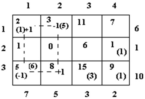
Consider the matrix giving the initial feasible solution for the problem under consideration. Let us start with any arbitrary empty cell (a cell without allocation), say        (3, 2) and allocate + 1 unit to this cell. As already discussed, in order to keep up the column 2 restriction, -1 must be allocated to cell (1, 2) and to keep up the row 1 restriction, +1 must be allocated to cell (1,1) and consequently -1 must be allocated to cell (3, 1); this is shown in the matrix below.

 

Table 

The net change in transportation cost as a result of this perturbation is called the evaluation of the empty cell in question.

Therefore,

Evaluation of cell (3,2)           = Rs.100 x (8 x 1 – 5 x 1 + 2 x 1 – 5 x 1)

                                             = Rs. (0 x 100)

                                             = Rs.0.

Thus the total transportation cost increases by Rs.0 for each unit allocated to cell (3,2). Likewise, the net evaluation (also called opportunity cost) is calculated for every empty cell. For this the following simple procedure may be adopted. 

Starting from the chosen empty cell, trace a path in the matrix consisting of a series of alternate horizontal and vertical lines. The path begins and terminals in the chosen cell. All other corners of the path lie in the cells for which allocations have been made. The path may skip over any number of occupied or vacant cells. Mark the corner of the path in the chosen vacant cell as positive and other corners of the path alternatively –ve, +ve, -ve and so on. Allocate I unit to the chosen cell; subtract and add 1 unit from the cells at the corners of the path, maintaining the row and column requirements. The net change in the total cost resulting from this adjustment is called the evaluation of the chosen empty cell. Evaluation of the various empty cells (in hundreds of rupees) are:

            Cell (1, 3) = c₁₃-c₃₃+c₃₁-c₁₁                  = 11-15+5       = -1,

            Cell (1, 4) = c₁₄-c₃₄+c₃₁-c₁₁                       =  7-9+5-2       = +1,

            Cell (2, 1) = c₂₁-c₂₄+c₃₄-c₃₁                       = 1-1+9-5        = +4,

            Cell (2, 2) = c₂₂-c₂₄+c₃₄-c₃₁+c₁₁-c₁₂     = 0-1+9-5+2-3 = +2,

            Cell (2, 3) = c₂₃-c₂₄+c₃₄-c₃₃                       = 6-1+9-15      = -1,

            Cell (3, 2) = c₃₂-c₃₁+c₁₁-c₁₂                       = 8-5+2-3        = +2.

 

If any cell evaluation is negative, the cost can be reduced so that the solution under consideration can be improved i.e., it is not optimal. On the other hand, if all cell evaluations are positive or zero, the solution in question will be optimal. Since evaluations of cells (1, 3) and (2, 3) are –ve, initial basic feasible solution given in table 3.15 is not optimal. 

Now in a transportation problem involving m rows and n columns, the total number of empty cells will be,

 m.n – (m+n-1) = (m-1) (n-1). 

Therefore, there are (m-1) (n-1) such cell evaluations which must be calculated and for large problems, the method can be quite inefficient. This method is named ‘stepping-stone’ since only occupied cells or ‘stepping stones’ are used in the evaluation of vacant cells.

2. Transportation Algorithm (Modified Distribution Method - MODI method) 

Various steps involved in solving any transportation problem may be summarized in the following iterative procedure:

Step1: Find the initial basic feasible solution by using any of three methods discussed above.

Step2: Check the number of occupied cells. If there are less than m+n-1, there exists degeneracy and it is possible to introduce a very small positive assignment of Î(»0) in suitable independent positions, so that the number of occupied cells is exactly equal to m+n+1.

Step 3:  For each occupied cell in the current solution, solve the system of equations

u_i+v_j=c_ij.

 Starting initially with some u_i=0 or v_j=0 and entering the successively the values of u_i and v_j in the transportation table margins. 

Step 4: Compute the net evaluation z_ij-c_ij=u_i+v_j-c_ij for all unoccupied basic cells and enter them in the upper right corners of the corresponding cells. 

Step 5: Examine the sign of each z_ij-c_ij. If all z_ij-c_ij £ 0 , then the current basic feasible solution is an optimum one. If atleast one z_ij-c_ij > 0, select the unoccupied cells, having the largest positive net evaluation to enter the basis. 

Step 6: Let the unoccupied cell (r,s) enter the basis. Allocate an unknown quantity, say q, to the cell (r,s). Identify a loop that starts and ends at the cell (r,s) and connects some of the basic cells. Add and subtract interchangeably, q  to and from the transition cells of the loop in such a way that the rim requirements remain satisfied.

Step 7: Assign a maximum value to q in such a way that the value of one basic variable becomes zero and the other basic variables remain non-negative. The basic cell whose allocation has been reduced to Zero, leaves the basis.

Step8: Return to step 3 and repeat the process until an optimum basic feasible solution has been obtained. 

3. Unbalanced Transportation Problem

For  a feasible solution to exist in a transportation problem, it is necessary that the total supply must equal demand. That is,  . But a situation may arise when the total available supply is not equal to the total requirement. Such type of transportation problem is called unbalanced transportation problem.

Problem:

Find the starting solution in the following transportation problem by any one of the methods (North-west Corner Method, Least–Cost Method, Vogel’s Approximation Method, Row minima method or column minima method).  Also obtain the optimum solution by using the best starting solution:

Source	Destination				Supply
	D1	D2	D3	D4
S1	3	7	6	4	5
S2	2	4	3	2	2
S3	4	3	8	5	3
Demand	3	3	2	2

 

Step 1: In this problem we find the basic feasible solution by using Vogel’s approximation method. 

By Vogel’s Approximation Method, the differences between the two successive lowest costs for each row and each column are computed.  These are written besides the corresponding rows or columns under the heading ‘row difference’ or ‘column difference”:

 

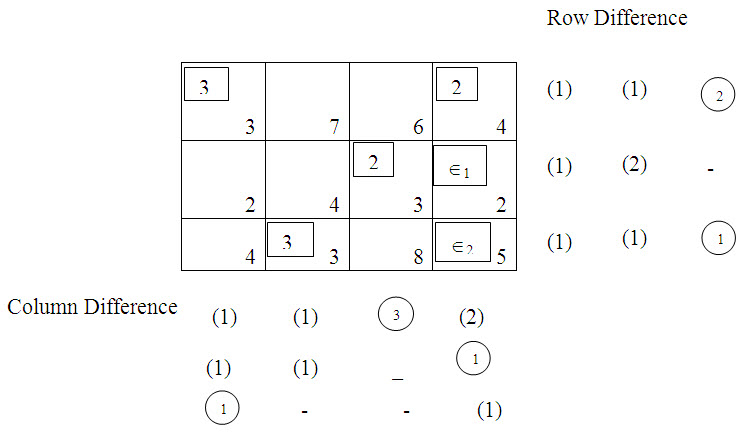
The largest row difference or column difference is 3 which corresponds to third column.  Allocating as much as possible to the lowest cost cell in the third column give x₂₃ = 2.  This satisfies the supply at S₂ and the requirement at D₃.  So arbitrarily we cross off the third column and consider e₁ (0) as the small quantity to be supplied form S₂.  The row and column differences are now recomputed for the reduced cost matrix, and  choose the largest of these, i.e., 2 which corresponds to fourth column.  Therefore allocate x₂₄ = e₁ and second row is now eliminated.  Again, compute the row and column differences for the reduced 2x3 transportation table and choose the largest of these, i.e., 4 corresponding to the second column.  Thus allocate x₃₂  = 3 and eliminate second column while consider  e₂ (0) being the negligible positive quantity to be supplied form S₃.  Again, computing the column and row differences in the reduced 2x2 cost matrix, we assign x₁₁ = 3 and thus eliminate first column.  This leaves now only fourth column, which can be filled by inspection and thus we assign x₁₄ = 2 and x₃₄e₂.

 

Step 2:  From the initial basic feasible solution obtained in step 1, it is observed that the best starting solution is obtained using Vogel’s approximation method having the least transportation cost of 32.  Also, observe that unknown quantities e_1, e₂ (> 0) have been allocated in the unoccupied cells (2,4) and (3,4) respectively to overcome the danger of degeneracy.

Step 3:  Now compute the numbers u_i (i = 1,2,3) and v_j (j = 1,2,3,4) using successively the equations u_i + v_j = c_ij for all the occupied cells.  For this it may be arbitrarily assigned as,  v₄ = 0.  Thus we have

                        u₁ + v₄ = c₁₄  u₁ + 0 = 4  u₁ = 4

                        u₂ + v₄ = c₂₄  u₂ + 0 = 2  u₂ = 2

                        u₃ + v₄ = c₃₄  u₃ + 0 = 5  u₃ = 5

Given u_1,u₂ and u₃, values of v_1,v₂ and v₃ can be calculated as shown below :

                        u₁ + v₁ = c₁₁  4 + v₁ = 3  v₁ = -1

                        u₂ + v₂ = c₂₃  2 + v₃ = 3  u₃ = 1

                        u₃ + v₃ = c₃₂  5 + v₂ = 3  v₂ = -2

The net evaluations for each of the unoccupied cells are now determined:

            z₁₂ – c₁₂ = u₁ + v₂ – c₁₂ = 4 + (-2) -7 = -5       

            z₁₃ – c₁₃ = u₁ + v₃ – c₁₃ = 4 + 1 -6 = -1           

            z₂₁ – c₂₁ = u₂ + v₁ – c₂₁ = 2 + (-1) - 2 = -1      

            z₂₂ – c₂₂ = u₂ + v₂ – c₂₂ = 2 + (-2) -4 = - 4      

            z₃₁ – c₃₁ = u₃ + v₁ – c₃₁ = 5 + (-1) –4 =  0

            z₃₃ – c₃₃ = u₃ + v₃ – c₃₃ = 5 + 1 -8 = -2           

Since all z_y - c_y £ 0, the current basic feasible solution is an optimum one.

It is possible to present a more compact form for computing the unknown u_t’s and v_j’s and then evaluate the net evaluations for each of the unoccupied cells in a more convenient way by working in the transportation table margins:

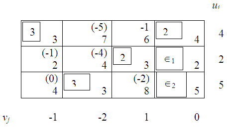
The optimum solution is:

x₁₁=3; x₁₄ = 2; x₂₃= 2; x₂₄=Î_1; x₃₂=3; x₃₄=Î_2.   

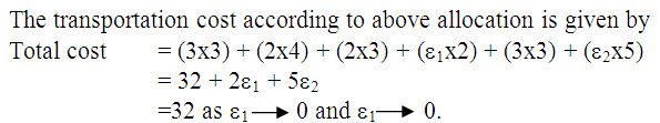
            The transportation cost associated with the optimum schedule is given by: 

            Total cost = (3x3) + (2x4) + (2x3) + (2x₁) + (3x3) + (5x₂)

                             = 32 + 2₁ + 5₂  

                             = 32, since ₁ → 0 and ₂ → 0.