Site pages
Current course
Participants
General
Module 1: Introduction and Concepts of Remote Sensing
Module 2: Sensors, Platforms and Tracking System
Module 3: Fundamentals of Aerial Photography
Module 4: Digital Image Processing
Module 5: Microwave and Radar System
Module 6: Geographic Information Systems (GIS)
Module 7: Data Models and Structures
Module 8: Map Projections and Datum
Module 9: Operations on Spatial Data
Module 10: Fundamentals of Global Positioning System
Module 11: Applications of Remote Sensing for Eart...
Lesson 10 Digital Image
10.1 Introduction to Digital Image
A digital image is a two dimensional array of discrete image elements or pixels representing spatial distribution of different parameters such as electromagnetic radiation, emission, temperature, or some geophysical or topographical elevation etc. Each pixel represented by a specific row (i) and column (j) value in an array or matrix. Each pixel associated with a pixel value is also called brightness value (BVij), represented as Digital Number (DN), which are stored as binary digits in a computer. This BVij’s represented in a gray level or gray scale is in certain ranges such as 0-255 (8-bit image: 28=256) in a black and white image. 0 and 255 represented as completely black and white respectively. For colour pictures three image matrices (as parallel layers) with same ranges are required. A single image can be represented as a black and white image in a two dimensional (2D) array (matrix) of pixels having rows (i) and columns (j). A multi-spectral or hyper- spectral image can be represented in a 3D array of pixels having rows (i), columns (j) and bands (k). Fig. 10.1. shows a digital image configuration of a single band.
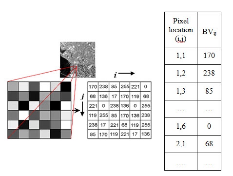
Fig. 10.1. Digital image configuration.
The features of the earth’s surface are imaged simultaneously by different sensors with filters corresponding to different wavelength bandwidth recorded as analog signal. This analog signal is converted in digital format using Analog to Digital converter and scale into different ranges like 8-bit (28=256), 9-bit (29=512), 10-bit (210=1024). A digital image is a data matrix having integer values representing the average of energy reflected/emitted from a square area on the surface of earth.
10.2 Image Rectification and Restoration
Remotely sensed images are taken from a great distance from the surface of the earth affected by various parameters such as atmosphere, solar illumination, earth rotation, sensor motion with its optical, mechanical, electrical components etc. which causes distortion in the imagery. The intent of image rectification and restoration is to correct these distortions arises in image acquisition process both geometrically and radiometrically. Obviously, the nature of such procedures varies considerably with factors such as the digital image acquisition type (digital camera, along-track scanner, across-track scanner), platform (airborne, satellite), atmosphere and total field of view.
10.3 Geometric Correction
Raw digital images acquired by earth observation systems usually contain geometric distortions so they do not reproduce the image of a grid on the surface faithfully. Geometric distortions are the errors in the position of a pixel relative to other pixels in the scene and with respect to their absolute position in a particular projection system.
The geometric distortions are normally two types: (i) systematic or predictable, and (ii) random or unpredictable.
Due to rotation of earth and platform’s forward motion the scan lines are not perpendicular to the direction of ground track, which makes the scanned area skewed and scale variation due to earth’s curvature found in both push-broom and whisk-broom scanner. But in case of whisk-broom scanner, there are additional two errors founds (a) scale variation along the scan direction due to its scanning process, (b) error due to nonlinearity in scan mirror velocity.
Random distortions and residual unknown systematic distortions are difficult to account mathematically. These are corrected using a procedure called rectification.
Rectification is process of correcting an image so that it can be represented on a plain surface. It includes the process known as rubber sheeting, which involves stretching and warping image to georegister using control points shown in the image and known control points on the ground called Ground Control Point (GCP). Rectification is also called georeferencing.
The image analyst must be able to obtain both the distinct sets of co-ordinates: image co-ordinates and map co-ordinates (x,y) associated with GCPs. These values are used in a least squares regression analysis to determine geometric transformation coefficients that can be used to interrelate the geometrically correct (map) coordinates and the distorted- image coordinates. The GCPs are chosen such that these can be easily identified on the image and whose geographic co-ordinates can be obtained from ground (using GPS) or from existing geo-referenced map or image. The two common geometric correction procedures generally used are: image-to-map rectification and image-to-image registration, which uses an existing georeferenced map and image correspondingly. Fig 10.2 shows rectified map which can be used to rectify an unrectified image.

Fig. 10.2. Image to map rectification.
Two basic operations are performed for geometric correction: (1) Spatial interpolation and (2) Intensity interpolation. Spatial interpolation accounts for the pixel position correction and intensity interpolation accounts for the DN value assignation from input image to its corresponding output pixel position.
(1) Spatial interpolation
The first process of geometric correction involves the pixel position correction using rubber sheeting procedure. The input and output image co-ordinate systems can be related as:
x= f1 (X, Y) and y = f2(X, Y) (10.1)
where,
(x, y) = distorted input image coordinates (column, row)
(X, Y) = correct image coordinates
f1, f2 = transformation functions
The mapping function could be polynomial. A first degree polynomial can model six kinds of distortions: translation and scale changes in x and y, skew and rotation.
The 1st degree polynomial (i.e. linear equation) can be mathematically expressed as
x = a0 + a1 X + a2 Y (10.2)
y = b0 + b1 X + b2 Y (10.3)
The co-efficients ai and bi are evaluated using GCPs.
(2) Intensity interpolation
Intensity interpolation involves the extraction of DN value from input image to locate it in the output image to its appropriate location. Fig 10.3 used as an example, for an output pixel (3, 5) grey shaded, the corresponding input pixel is (2.4, 4.8). This means the output image may not have one-to-one match with the input image. Therefore an interpolation process is applied which is known as resampling. This process accounts the position of output pixel to its corresponding position of input pixel and the DN values of input pixel and their surroundings.
![]()
Fig. 10.3. a) Distorted image; b) Corrected image pixels matrix.
There are generally three kinds of resampling process-
a) Nearest-neighbour interpolation
Let for an output pixel (3, 5), in Fig 10.3 the input pixel location is (2.4, 4.8). In nearest-neighbor interpolation, the output pixel (3, 5) will be filled up with DN value nearest to the input pixel location (2.4, 4.8) in the present case is (2, 5). In this process the radiometric values or DN values do not alter and it is computationally efficient. But features in the output matrix may be offset spatially by + 0.5 pixel, thus a ‘patchy’ appearance arise at the edges and in linear features.
b) Bilinear interpolation
Bilinear interpolation finds brightness values in two orthogonal direction of the desired input location (2.4, 4.8) in the input image. Distance-weighted average of DN values of four nearest pixels ((1, 4), (1, 5), (2, 4), (2, 5)) is computed in the input distorted image. Closer to the input location will have more weight; DN value of highest weighted pixel will be assigned to the output pixel.
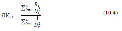
where, Rk are the surrounding four DN values, D2k are the distance squared from the desired input location (2.4, 3.8).
This technique alters the DN value and generates smoother appearance in the resampled image.
c) Cubic convolution interpolation
An improved restoration of the image is obtained in cubic convolution interpolation process. Similar to bilinear interpolation this technique is uses 16 neighbor pixel in the input image. It provides smoother appearance and sharpens edge and also changes the DN values but requires more computational time than previous processes.
Any interpolation is a low pass filtering operation and it produces a loss of higher frequency information depending on the method used.
10.4 Radiometric Correction and Noise Removal
Radiance value recorded for each pixel represents the reflectance/emittance property of the surface features. But the recorded value does not coincide with the actual reflectance/ emittance of the objects due to some factors like: sun’s azimuth and elevation, viewing geometry, atmospheric conditions, sensor characteristics, etc. To obtain the actual reflectance/ emittance of surface features, radiometric distortions must be compensated. The main purpose of radiometric correction is to reduce the influence of errors. An error due to sensor’s characteristic is also referred as noise.
Radiometric correction is classified into the following three types:
1) Sun angle and topographic correction
2) Atmospheric correction
3) Detector response calibration
a) De-striping
b) Removal of missing scan line
c) Random noise removal
d) Vignetting removal
1) Sun angle and topographic correction: The sun elevation correction accounts for the seasonal position of the sun relative to the earth (Fig. 10.4). The correction is usually applied by dividing each pixel value in a scene by the sine of the solar elevation angle or the cosine of zenith angle (which is simple 900 minus the solar elevation angle).
DNcorrection = DN / sinα (10.5)
DNcorrection = DN / cosθ (10.6)
α = solar elevation angle, θ = zenith angle (90o- elevation angle)
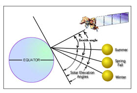
Fig. 10.4. Effects of seasonal changes on solar elevation angle.
(Source: landsathandbook.gsfc.nasa.gov/data_properties/prog_sect6_3.html; and modified )
The earth- sun distance correction is applied to normalize for the seasonal changes in the distance between the earth and the sun. The earth- sun distance is usually expressed in astronomical units. (An astronomical unit is equivalent to the mean distance the earth and the sun, approximately 149.6×10⁶km). The irradiance from the sun decreases as the square of the earth-sun distance (Lillesand and Kiefer, 2003).
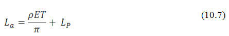
2) Atmospheric correction: During transmission of EM wave from sun to objects and from objects to sensor through atmosphere, various kinds of absorption and scattering takes place. Objects receive not only the direct solar illumination, but also the scattered radiation from atmosphere and neighbouring objects and similarly the sensor receives reflection or radiation from target, its neighbouring objects, and scattered radiation from atmosphere (which is called path radiance or haze).
Therefore the sensor receives a composite reflection/ radiation which can be expressed as-
where,
La = apparent spectral radiance
measured by sensor
ρ = reflectance of objects
E = irradiance on object
T = transmission of atmosphere
Lp = path radiance / haze
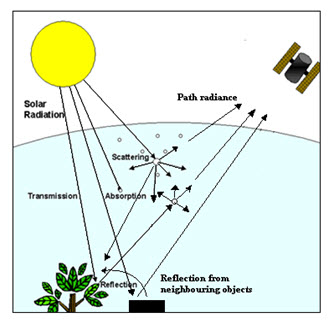
Fig. 10.5. Effect of solar illumination in atmosphere
For multispectral and hyperspectral data, the approaches of atmospheric correction is different.
The errors due to solar elevation, sun-earth distance and atmospheric effects can be reduced in two procedures: (i) absolute correction and (ii) relative correction.
Absolute correction
The absolute correction procedure of Landsat data is stated below:
The radiance recorded by a sensor is converted in DN values in a range 0 – 255 (in 8 bit data). Therefore to obtain reflectance value of terrain objects it is required to convert DN values back to its equivalent the radiance value, and radiance value to reflectance value.
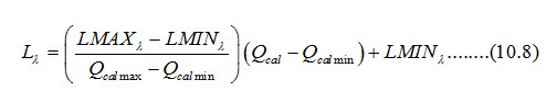
where,
Lλ = Spectral radiance at the sensor’s aperture
LMAX λ = Spectral at-sensor radiance that is scaled to Qcal min.
LMIN λ = Spectral at-sensor radiance that is scaled to Qcal max.
Qcal= Quantized calibrated pixel value (DN).
Qcal max= Maximum quantized calibrated pixel value corresponding to LMIN λ.
Qcal min= Maximum quantized calibrated pixel value corresponding to LMAX λ.
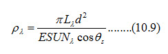
where,
ρλ = TOA reflectance
Lλ = Spectral radiance at the sensor’s aperture
d= Earth-Sun distance
ESUNλ= Mean exoatmospheric solar irradiance
θs= Solar zenith angle
The values of Lλ, LMAXλ, LMINλ, Qcal, Qcal max, Qcal min, θs are obtained from the sensor parameters and satellite position.
Table 10.1 Solar spectral irradiances for bands of ETM+ sensor
|
Band |
watts/(meter squared * µm) |
|
1 |
1969.000 |
|
2 |
1840.000 |
|
3 |
1551.000 |
|
4 |
1044.000 |
|
5 |
225.700 |
|
7 |
82.07 |
|
8 |
1368.000 |
(Source: landsathandbook.gsfc.nasa.gov/data_prod/prog_sect11_3.html)
Table 10.2 Earth-Sun distance in astronomical units
|
Julian Day |
Distance |
Julian Day |
Distance |
Julian Day |
Distance |
Julian Day |
Distance |
Julian Day |
Distance |
|
1 |
0.9832 |
74 |
0.9945 |
152 |
1.0140 |
227 |
1.0128 |
305 |
0.9925 |
|
15 |
0.9836 |
91 |
0.9993 |
166 |
1.0158 |
242 |
1.0092 |
319 |
0.9892 |
|
32 |
0.9853 |
106 |
1.0033 |
182 |
1.0167 |
258 |
1.0057 |
335 |
0.9860 |
|
46 |
0.9878 |
121 |
1.0076 |
196 |
1.0165 |
274 |
1.0011 |
349 |
0.9843 |
|
60 |
0.9909 |
135 |
1.0109 |
213 |
1.0149 |
288 |
0.9972 |
365 |
0.9833 |
(Source:landsathandbook.gsfc.nasa.gov/data_prod/prog_sect11_3.html)
Noise Removal: Image noise is any unwanted disturbance in image data that is due to limitations in the sensing, signal digitization, or data recording process. Radiometric errors due to detector response calibration are also termed as noise.
3) Detector response calibration
Destriping: Striping or banding in imagery occurs due to error in sensor adjustment or inability in sensing the radiation by sensors. This error was common in Landsat MSS sensor, where six detectors were used for each band drifted over time, resulting in relatively higher or lower values along every sixth line in the image. One common method of striping error correction is done by comparing the histogram between a set of data. A histogram is evaluated from scan lines 1, 7, 13, and so on; for a second lines 2, 8, 14, and so on; and so forth. These histograms are then compared in terms of their mean and standard deviations of six detectors to identify the problem detector(s) for the problem lines to resemble those for the normal data lines. Fig. 10.6(a) shows a stripped image and Fig. 10.6(b) is the output result after de-striping algorithm is applied.
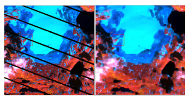
Fig. 10.6. Destriping: (a) striped image, (b) destriped image.
(Source: blamannen.wordpress.com/2011/07/12/destripe-landsat-7-etm-some-thoughts/)
Line drop: Line drop correction is similar to strip error. Line drop error is found when a sensor completely fails to scan. This can be minimized by normalizing with respect to their neighboring features or image values i.e. the data for missing lines is replaced by the average image value of neighbors. Fig. 10.7 shows the line drop correction.
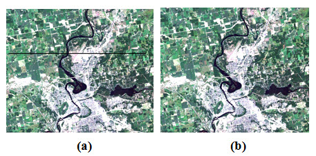
Fig. 10.7. Line drop correction: (a) original image (b) restored image.
Random noise removal: Random noise is not systematic. The noise in a pixel does not depend on the spatial location of the pixel in the imagery. It causes images to have a “salt and pepper” or “snowy” appearance. Moving window of 3 x 3 or 5 x 5 pixels is used for removing these errors.
Vignetting removal: Vignetting is found when the central portion image is more brighten than the periphery or corners. This error is found in images obtained from optical sensor, which uses lens. Images taken using wide-angle lenses often vignette due to refraction property of light. Proper calibration between the irradiance and sensor output signal is generally used for this correction. Fig. 10.8. shows the vignetting effect in left image and the right image is the output after vignetting removal is applied.
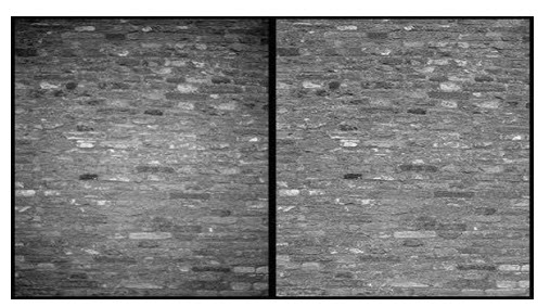
Fig. 10.8. Left image have vignetting effect in contrast to the uniform image.
(Source: www.rbc.ufrj.br/_pdf_56_2004/56_1_06.pdf)
Keywords: Digital image, Rectification, Geometric correction, Radiometric correction, Noise.
References
blamannen.wordpress.com/2011/07/12/destripe-landsat-7-etm-some-thoughts/
geoinformatics.sut.ac.th/sut/vichagan/DIP/Chapter_07.pdf
landsathandbook.gsfc.nasa.gov/data_properties/prog_sect6_3.html
landsathandbook.gsfc.nasa.gov/data_prod/prog_sect11_3.html
Lillesand, T. M., Kiefer, R. W., 2002, Remote sensing and image interpretation, Fourth Edition, pp. 471-488.
www.rbc.ufrj.br/_pdf_56_2004/56_1_06.pdf
www.wamis.org/agm/pubs/agm8/Paper-5.pdf
Suggested Reading
Bhatta, B., 2008, Remote sensing and GIS, Oxford University Press, New Delhi, pp. 311-322.
Joseph, G., 2005.Fundamentals of Remote Sensing, Second Edition, Universities Press (India) Pvt. Ltd., pp. 320-321.
nature.berkeley.edu/~penggong/textbook/chapter5/html/sect52.htm
www.e-education.psu.edu/natureofgeoinfo/book/export/html/1608
Last modified: Friday, 24 January 2014, 5:51 AM