Remote Sensing & GIS Applications 3(2+1)

Lesson 11 Pre Processing Techniques

11.1 Image Reduction and Image Magnification

11.1.1 Image Reduction

Sometimes it is necessary to view the entire image in more detail e.g. for visual interpretation. Many image processing systems are not able to display the full image containing rows and column greater than 3000 and 3000 respectively. Let a study area be covered by 5028 x 4056 pixels. In such circumstances, image reduction allows the viewers to display the full image, which also reduces the image dataset to a smaller dataset. This technique is useful for orientation purposes as well as delineating the exact row and column coordinates of an area of interest. To reduce a digital image to just 1/m squared of the original data, every mth row and mth column of the image are systematically selected and displayed. If m=2 is used; this will create a 2x reduced image containing 2514 x 2028 (= (5024/2) x (4056/2)) rows and columns respectively. This reduced image would contain only 25% of the pixels found in the original scene. The procedure of 2x reduction is shown in Fig. 11.1.

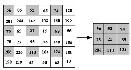
Fig. 11.1. Image reduction (2x).

In Fig. 11.1, every second row and second column is sampled. Thus a 2x reduction means every second row and second column of the original image will be sampled. A sample image reduction in 2x and 4x is shown in Fig. 11.2.

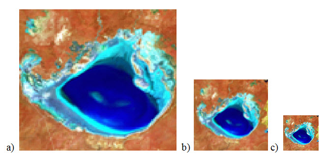
Fig. 11.2. a) Original image, b) 2x reduced image, c) 4x reduced image.

11.1.2 Image Magnification

Digital image magnification is often referred to as zooming. It improves the scale of the image for enhanced visual interpretation. In image reduction pixels are deleted depending on the order of reduction and image magnification is done by replication of rows and columns.

To magnify an image by an integer factor n squared, each pixel in the original image is usually replaced by an n X n block of pixels all of which have the same pixel values as the original input pixel. The logic of a 2x magnification is shown in Fig. 11.3. This form of magnification doubles the size of each of the original pixel values. An example of magnification is shown in Fig. 11.4

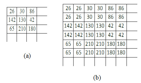
Fig. 11.3. a) Original image,  b) 2x magnified image.

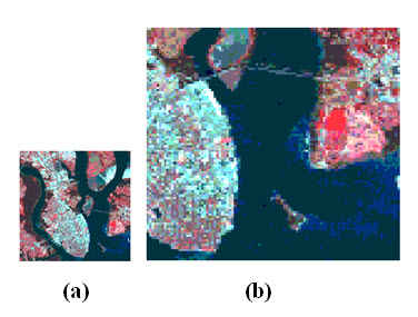
Fig. 11.4. a) Original image, b) 2x magnified image.

(Source: www.uriit.ru/japan/Our_Resources/Books/RSTutor/Volume3/mod7/7-1/7-1.html)

11.2 Color Compositing

In displaying a color composite image three primary colors (red, green, and blue) are used. Thus to create a colour image three bands of multi-band image is required. These three bands is passed through the primary color gun, creates a color image. Different color images may be obtained depending on the selection of three-band images and the assignment of the three primary colors. Color intensity of a feature in an image depends on the spectral reflectance of that feature in the three selected bands.

True colored image is said to the image, which shows the features in their actual color. Multispectral image dataset contains spectral bands in the red, green, and blue spectrum region of the electromagnetic (EM) spectrum, may be combined to produce a true color image. True colored image can be obtained by passing the red band through red color gun, green band through green color gun, and blue band through blue color gun of a display system. Landsat ETM+, IKONOS image dataset are example of multispectral image dataset contains red, green, and blue bands.

Human eye is able to see the radiation having wavelength within the visual portion of the electromagnetic spectrum. Thus to see the radiations having wavelength lying out of the visible portion of the electromagnetic spectrum, False Color Composite (FCC) is required. In this case, spectral bands like Infrared (IR), Near-Infrared (N-IR), Thermal Infrared (T-IR) etc. are pass through the visual color gun to see the reflection/ radiation of features in these bands. Thus obtained image is known as FCC image. If the N-IR band radiation passes through the red color gun, red through green, and green through blue; thus obtained image is known as Standard FCC image. Compared to true color image, in standard FCC the vegetation appears better depending on the types and conditions, since vegetation reflects much in N-IR region of the EM spectrum than the green. As N-IR band passes through red color gun, vegetation appears red in Standard FCC image (Fig. 11.5).

Spectral bands of image datasets which do not contain three visible bands (IRS LISS-III/ LISS-IV or SPOT HRV) are mathematically combined resembles to a true color image, can be produced as follows:

RED colour gun = Red

GREEN colour gun = (3* Green + NIR)/4 = 0.75*Green + 0.25*NIR

BLUE colour gun = (3* Green - NIR)/4 = 0.75*Green - 0.25*NIR

In practice, we use various color combinations to facilitate the visual interpretation of an image depending on the nature of application and reflection/ radiation property of surface features.

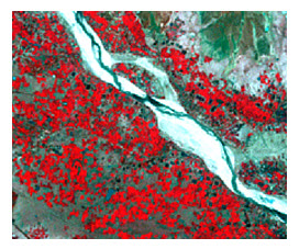
Fig. 11.5. False colour composite multispectral Landsat TM image.

11.3 Image Enhancement

Image enhancement procedures are applied to original image data to improve the quality of image, which would be more suitable in image interpretation and feature extraction depending on the nature of application. Although radiometric corrections are applied, the image may still not be optimized for highest level of visual interpretation. Thus it increases the amount of information that can be extracted visually. The image enhancement techniques are applied either to single-band images or separately to the individual bands of a multi-band image set. There are numerous procedures that can be performed to enhance an image. However, they can be achieved using two major functions: global operations (spectral or radiometric enhancement) and local operations (or spatial enhancement). Global operations change the value of each individual pixel independent of neighbor pixels, while local operations change the value of individual pixels in the contest of the values of neighboring pixels.

Global Operation or Radiometric Enhancement

Contrast is the relative brightness in DN values or radiometric values. Object distinction in high contrast image is more suitable than low contrast image, as our eyes are good in discriminating higher radiometric differences. Thus the contrast or radiometric enhancement is used to improve the radiometric differences between the objects for better visual interpretability. It can normally categorized as

1)    Grey level thresholding

2)    Density slicing

3)    Contrast stretch

1) Gray-Level Thresholding

Gray- level thresholding is used to segment an input image into two classes one for those pixels having DN values below an analyst defined value and another for those above this value. Thus thresholding on an image creates a binary image contains pixels of only two DN values, 0 and 255. In following example (Fig. 11.6.), let threshold value 185 is applied. In the input image, all the pixels having DN values less than 185 will appear pure black (DN value=0) and all the pixels having DN values greater than 185 will appear white (DN value=255) in the output image.

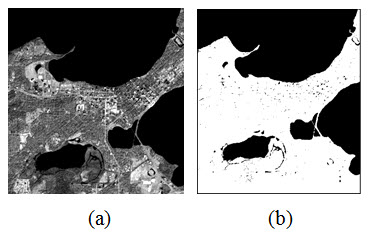
Fig. 11.6. a) Input Image b) Output image after thresholding.

2) Density or Level Slicing

Level slicing is similar to grey level thresholding. In grey level thresholding, the input image pixels are segmented in two groups lower and higher of a defined DN value or level, in case of level slicing a number of levels (m) are used, which segmented the image in a numbers of groups (m+1). Thus in density slicing or level slicing, the image histogram is divided into an analyst specified intervals or slices. All of the DN values in the input image falling within a specified are then displayed at a single DN in the output image. Consequently, if four slices are established, the output image will contain four different gray levels (Fig 11.7).

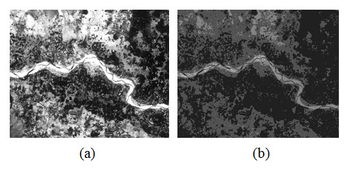
Fig. 11.7. a) Input image b) Output image (having 4 slices).

Application of density slice reduces the details of an image, but it also reduces the noise in the image. This is useful in highlighting the features in the imagery.

Histogram: Histogram is a graphical presentation of DN value of a pixel and occurrence of pixels having same DN value (frequency) in an image.  From the histogram of an image the contrast of an image can easily be understood. In low contrast image the radiometric differences or differences in DN values are less, and in high contrast image the radiometric differences or differences in DN values are high (Fig. 11.8).

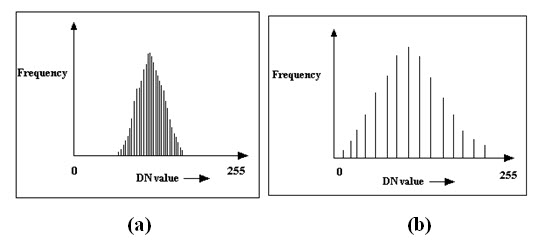
Fig. 11.8. a) Low contrast histogram b) high contrast histogram

3) Contrast Stretching

One of the most useful method of contrast enhancement is contrast stretching. 8 bit image data contains 256 (=2⁸) levels in grey scale of DN values. Often remote sensing sensors fail to collect reflectance/radiation covering the entire 256 levels, normally confined to a narrow range of DN values, which produce a low contrast image. Let an input image have brightness values between 60 and 158. Contrast stretching operation expands the narrow range (60 to 158) of DN values of the input image to the full range (0 to 255) of DN values in the output image.

Contrast stretch is categorized as a) linear and b) non-linear.

a) Linear Contrast Stretch

In linear contrast stretch the input histogram is stretched uniformly. Thus it drags the minimum DN value to the zero (0; the lowest grey level of display system) and maximum DN value to the 255 (the highest grey level of the display system) and stretch all the interlaying DN values uniformly. This uniform expansion is called a linear stretch. This increase the contrast of an image, therefore subtle variations in input image date values would now be displayed in output tones that would be more readily distinguishable by an interpreter. Light tonal areas would appear lighter and dark areas would appear darker. An example of linear contrast stretch is shown in Fig. 11.9.

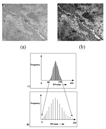
Fig. 11.9. a) Original image, b) after linear contrast stretch, c) input histogram, d) output histogram.

The linear contrast stretch would be applied to each pixel in the image uses the algorithm

where,

DN' = digital number assigned to pixel in output image

DN = original digital number of pixel in input image

MIN = minimum value of input image, to be assigned a value of 0 in the output image (60 in the above example)

Max = maximum value of input image, to be assigned a value of 255 in the output image (158 in the above example).

b) Non-linear Contrast Stretch

One drawback of the linear stretch is that it assigns as many display levels to the rarely occurring DN values as it assigns as many occurring values. Due to uniform radiometric enhancement, the stretch between DN values in the both tails (zones of low frequency DN values) is equal to the middle of the histogram (zones of high frequency DN values). The low frequency means less number of pixels, which is less important for information extraction, gets equal importance in the linear contrast enhancement operation. To avoid this, non-linear contrast stretch is applied to the image data.

Histogram equalization- One method of non-linear contrast stretch is histogram equalization (shown in Fig. 11.10.), in which the contrast stretching depends on the histogram of the image data. The contrast stretch will be higher between the DN values having higher frequency than the lower frequency DN values. But it suppresses the lower frequency pixels, which have less subject to interest.

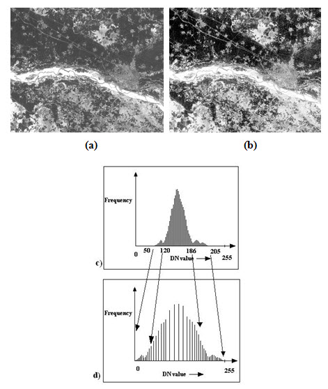
Fig. 11.10. a) Original image, b) output image after histogram equalization, c) input image histogram, d) output image histogram.

As shown in Fig. 11.10., in the input histogram greater display values (and hence more radiometric detail) are assigned to the frequently occurring portion of the histogram. The image value range of 120 to 186 (high frequency) is stretched more than lower value range 50 to 120 (low frequency) and 186 to 205 (low frequency).

Local Operations or Spatial Enhancement

Spatial image enhancement is used to increase the image quality through filtering. Spatial frequency is the rate of change of image values or DN values in the scene in a unit distance. Filtering operation emphasizes or de-emphasizes this spatial frequency for better image interpretation. Thus filters highlight or suppress specific features based on their spatial frequency hence it depends on the image value of neighbors. Different kinds of filters are explained below.

Convolution filter: In convolution filtering a window also known as operators or kernels having odd numbers of pixels (e.g., 3x3, 5x5, 7x7) used to move throughout the input image, the DN value of the output image is obtained by a mathematical manipulation. A convolution filter is classified as low-pass filter and high-pass filter.

Low-pass filter: A low-pass filter emphasizes low frequency or homogeneous areas and reduces the smaller details in the image. It is one of the methods of smoothing operation. It reduces the noise in the imagery. Low-pass filter normally sub-divided as average (mean), mode and median filter.

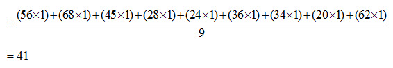
Average filter: In case of average or mean filter the output DN value is obtained by multiplying each coefficient of the kernel with the corresponding DN in the input image and adding all them all and dividing by the sum of kernels value.  The coefficients of the kernel range from equal value to different weighted value.

Mode filter: A kernel is fitted in the input image, and computes the mode value within this kernel. The resultant value is the final value of the center pixel of the kernel.

Median filter: Median filter is similar to mode filter. In this case the median value of the kernel is computed which replaces the center pixel DN value. Median filter is very useful for removing random noise, salt-pepper pattern noise, speckle noise in RADAR imagery.

High-pass filter: High-pass filter is the opposite of low-pass filter. In contrast to low-pass filter, high-pass filter enhance the variations in the imagery. It increases the spatial frequency, thus sharpens the details in the imagery. High frequency filter works in the similar way of average filter, uses a kernel may be normal or weighted. Another way of getting the output of high-pass filtering is subtraction of the low-pass filtered image from the original image. The following 5x5 image explains the operation of low pass and high pass filters.

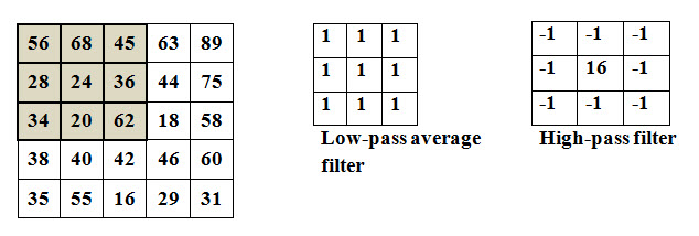
For, low-pass average filter, the central value of the of window in the output image will be

Similarly, if the high filter is applied, the calculated value will be 39, which will replace the value 24.

In the above example, the image values of the 3x3 window of the input image can be written in increasing order as 20, 24, 28, 34, 36, 45, 56, 62, 68. In this set 45 in the median value, this will replace the central kernel value 24. Similarly if a set of values of a 3x3 kernel is, as example 50, 62, 58, 20, 145, 19, 20, 96, 204, then the central kernel of the output image will be the mode value of the set, i.e. 20.

Edge Enhancement filter: Edge enhancement is quite similar to high frequency filter. High frequency filter exaggerate local brightness variation or contrast and de-emphasize the low frequency areas in the imagery. In contrast to this, edge enhancement filter emphasize both the high frequency areas along with low frequency areas. Is enhances the boundary of features. Different kinds of kernels are used depending on the roughness or tonal variation of the image.

Edge Detection filter: There may arise confusion with edge enhancement filter with edge detection filter, which highlights the boundary of the features and de-emphasizes the low contrast areas totally. It highlights the linear features such as road, rail line, canal, or feature boundary etc. Sobel, Prewitt and Laplacian etc filters are the example of edge detection filter. Fig. 11.11 shows image filtering operations using low pass, high pass, edge enhancement and edge detection filters.

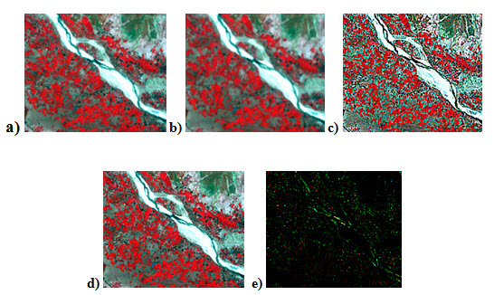
Fig. 11.11. a) Original image, output image applying: b) low pass filter, c) high pass filter, d) edge enhancement filter, e) edge detection filter.

Fourier Transform: The filters discussed above are spatial filters. Fourier analysis or transform the spatial domain is transferred to frequency domain. The frequency domain is represented as a 2D scatter plot, known as Fourier domain, where low frequencies falls at the center and high frequencies are progressively outward. Thus Fourier spectrum of an image can be used to enhance the quality of an image with the help of the low and high frequency block filters. After filtering the inverse Fourier transformation gives the output of the Fourier transformation. Fig. 11.12 shows the resulting images of application of Fourier spectrum and inverse Fourier spectrum.

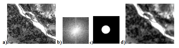
Fig. 11.12. a) Original image, b) Fourier spectrum of input image, c) Fourier spectrum after application of low pass filter, d) Output image after inverse Fourier transformation.

11.4 Image Manipulation

Each of the images acquired were manipulated in different ways to highlight various aspects of them.

These manipulations include mainly:

  Band ratioing

  Indexing

  Principal Component Analysis

Spectral Ratioing

Radiance or reflectance of surface features differs depending on the topography, shadows, seasonal changes in solar illumination angle and intensity. The band ratio of two bands removes much of the effect of illumination in the analysis of spectral differences. Ratio image resulting from the division of DN values in one spectral band by the corresponding values in another band. In the scene, there are mainly two types of rocks which are discernable in Fig. 11.13. b) but not in Fig. 11.13.a).

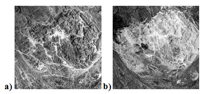
Fig. 11.13. a) Blue band shows topography due to illumination difference, b) ratio of band3/band2 removes illumination and yield different rock types.

(Source:geology.wlu.edu/harbor/geol260/lecture_notes/Notes_rs_ratios.html)

It should be kept in mind that different materials with different absolute radiances but having similar slopes may appear identical in band ratio image. One very useful band ratio image in vegetation monitoring is Ratio Vegetation Index (RVI) can be formulated as follows:

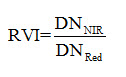
Indexing

Indexing is similar to band ratio. In contrast to band ratio or simple ratio, indexing is useful for nonlinear variation, thus overcome the discrepancy of misinterpretation sometime occurs in band ratio. As an example, Normalized Difference Vegetation Index (NDVI) uses the NIR and red bands; where the vegetation areas yield very high values because of high reflectance in NIR and low reflectance in visible band; whereas, clouds, water, snow yield negative index value and rock, bare soils etc. have very low or near zero index value (Fig. 11.14). Thus NDVI is very commonly used index in vegetation monitoring.

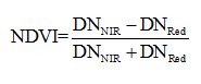
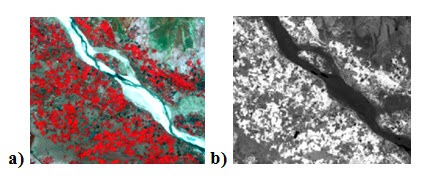
Fig. 11.14. a) FCC image of an area, b) NDVI output image; vegetation appears bright, river or wet land appears dark.

Principal Component Analysis

Spectral bands of multispectral data are highly correlated. Due to this high correlation in bands, the analysis of the data sometimes becomes quite difficult; thus images obtained by combining different spectral bands looks similar. To decorrelate the spectral bands, Principal Component Analysis (PCA) or Principal Component Transformation (PCT) is applied. PCA also have the capability of dimension reduction, thus PCA of a data may be either an enhancement operation prior to visual interpretation or a preprocessing procedure for further processing. Principal components analysis is a special case of transforming the original data into a new coordinate system. It enhances the subtle variation in the image data, thus many features will be identified which cannot be identifiable in raw image (Fig 11.15).

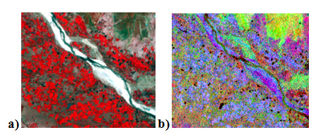
Fig. 11.15. a) Input image (RGB:432) b) output image (RGB: 432)

Keywords: Image reduction, Image magnification, Color composing, Image enhancement, Histogram equalization, Filtering, Fourier transform, PCA.

References

• geology.wlu.edu/harbor/geol260/lecture_notes/Notes_rs_ratios.html

• www.uriit.ru/japan/Our_Resources/Books/RSTutor/ Volume3/mod7/7-1/7-1.html

Suggested Reading

• Bhatta, B., 2008, Remote sensing and GIS, Oxford University Press, New Delhi, pp. 323-350.

• Lillesand, T. M., Kiefer, R. W., 2002, Remote sensing and image interpretation, Fourth Edition, pp. 471-532.

• www.gisknowledge.net/topic/ip_in_the_spatial_domain/smith_trodd_spatial_domain_enhance_07.pdf

• www.fas.org/irp/imint/docs/rst/Sect1/Sect1_13.html

• www.nrcan.gc.ca/earth-sciences/geography-boundary/remote-sensing/fundamentals/2187; 23 Dec., 2012