Remote Sensing & GIS Applications 3(2+1)

Lesson 19 Data Model Classification

19.1.1 Data quantization and storage

The range of values that can be stored by image pixels depends on the quantization level of the data, i.e. the number of binary bits used to store the data. The more the number of bits, the greater the range of possible values. The most common image data quantization formats are 8 bit and 16 bit. The binary quantization level selected depends partly on the type of data being represented and what it is used for. In many cases, the image data file contains a header record that stores information about the image, such as the number of rows and columns in the image, the number of bits per pixel and the geo referencing information. The main issue in connection with raster data storage is the disk space potentially required. The goal of raster compression is then to reduce the amount of disk space consumed by the data file while retaining the maximum data quality.

19.1.2 Spatial variability

The raster data model can represent discrete point, line and area features but is limited by the size of the pixel and by its regular grid-form nature. A point’s value would be assigned to and represented by the nearest pixel; similarly, a linear feature would be represented by a series of connected pixels; and an area would be shown as a group of connected pixels that most closely resembles the shape of that area.

19.1.3 Representing spatial relationships

Because the raster data model is a regular grid, spatial relationships between pixels are implicit in the data structure since there can be no gaps or holes in the grid. Each raster is referenced at the top-left corner; its location is denoted by its row and column position and is usually given as 0, 0. All other pixels are thenidentified by their position in the grid relative to the topleft. The upper left pixel being used as the reference point for ‘raster space’ is in contrast to ‘map space’ where the lower left corner is the geographical coordinate origin; this difference has an effect on the way raster images are geo referenced. Another benefit of implicit spatial relationships is that spatial operations are readily facilitated.

19.1.4 The effect of resolution

The accuracy of a map depends on the scale of that map. In the raster model the resolution, scale and hence accuracy depends on the real-world area represented by each pixel or grid cell. The pixel can be thought of as the limit beyond which the raster becomes discrete, and with computer power becoming ever greater we may have fewer concerns over the manageability of large, high-resolution raster files. Providing we maintain sufficient spatial resolution to describe adequately the phenomenon of interest, we should be able to minimize problems related to accuracy.

19.1.5 Representing surfaces

Raster’s are ideal for representing surfaces since a value, such as elevation, is recorded in each pixel and the representation is therefore ‘continuously’ sampled across the area covered by the raster. The input dataset representing the surface potentially contributes two pieces of information to this kind of perspective viewing. The first is the magnitude of the DN which gives the height and the second is the way the surface appears or is encoded visually, i.e. the DN value is also mapped to colour in the display. [(Liu, and Mason, 2009) Essential Image Processing and GIS for Remote Sensing, UK.]

(A) Advantage of Raster Data

• The geographic location of each cell is implied by its position in the cell matrix. Accordingly, other than an origin point, e.g. bottom left corner, no geographic coordinates are stored.

• Due to the nature of the data storage technique data analysis is usually easy to program and quick to perform.

• The inherent nature of raster maps, e.g. one attribute maps, is ideally suited for mathematical modeling and quantitative analysis.

• Discrete data, e.g. forestry stands, is accommodated equally well as continuous data, e.g. elevation data, and facilitates the integrating of the two data types.

• Grid-cell systems are very compatible with raster-based output devices, e.g. electrostatic plotters, graphic terminals.

(http://bgis.sanbi.org/gis-primer/page_19.htm Accessed on 03.12.2012.)

(B) Disadvantage of Raster Data

• The cell size determines the resolution at which the data is represented.

• It is especially difficult to adequately represent linear features depending on the cell resolution. Accordingly, network linkages are difficult to establish.

• Processing of associated attribute data may be cumbersome if large amounts of data exist. Raster maps inherently reflect only one attribute or characteristic for an area.

• Since most input data is in vector form, data must undergo vector-to-raster conversion. Besides increased processing requirements this may introduce data integrity concerns due to generalization and choice of inappropriate cell size.

• Most output maps from grid-cell systems do not conform to high-quality cartographic needs.

19.2 Vector Data

Vector data is a series of discrete features described by their coordinate positions rather than graphically or in any regularly structured way. Tabular data represent a special form of vectordata which can include almost any kind of data, whether or not they contain a geographic component.  Tabular data are not necessarily spatial in nature. The vector model could be thought of as the opposite of raster data in this respect, since it does not fill the space it occupies; not every conceivable location is represented, only those where some feature of interest exists.

There have been a number of vector data models developed over the past few decades, which support topological relationships to varying degrees, or not at all. The representation, or not, of topology dictates the level of functionality that is achievable using those data. These models include spaghetti (unstructured), vertex dictionary, dual independent map encoding (DIME) and arc-node (also known as POLYVRT). To understand the significance of topology it is useful to consider these models, from the simplest to the more complex.

19.2.1 Unstructured or spaghetti data

Spaghetti form of vector data is stored without relational information. There is no mechanism to describe how there features relate to one another i.e. there is no topology. The advantages of unstructured data are that their generation demands little effort and that the plotting of large unstructured vector files is potentially faster than the structured data. Disadvantages are that storage is insufficient.

19.2.2 Vertex dictionary

Vertex dictionary is a minor modification of the ‘spaghetti’ model. It involves the use of two files to represent the map instead of one. This prevents duplication, since each coordinate pair is stored only once, but it does not allow any facility to store the relationships between the features, i.e. topology is still not supported.

19.2.3 Dual Independent Map Encoding (DIME)

The DIME structure was developed by the US Bureau of the Census for managing its population Databases. Both street addresses and UTM coordinates were assigned to each entity in the database. Here again, additional files (tables) are used to describe how the coordinate pairs are accessed and used.

19.2.4 Arc-node Structure or “POLYVRT” (POLYgonconVeRTer)

A more efficient model for the storage of vector data, and one which supports topological relationships, is the ‘arc-node’ data structure. Here vector entities are stored separately but are linked using pointers. An arc is a line which, when linked with other arcs, forms a polygon. Arcs may be referred to as edges and sometimes as chains. A point where arcs terminate or connect is described as a node. Polygons are formed from an ordered sequence of arcs and may be termed ‘simple’ or ‘complex’ depending on their relationship to other polygons. When the features are digitized each arc is digitized between nodes, in a consistent direction; it has a start node, and is a given identifying number.

19.2.5 Connectivity

Connectivity allows the identification of a pathway between two locations, between your home and the airport, along a bus, rail and/or underground route,for instance. Using the arc-node data structure, a route along an arc will be defined by two end points, the start or from-node and the finish or to-node. Network connectivity is then provided by an arc node list that identifies which nodes will be used as the from and to positions along an arc

19.2.6 Area Definition

This is the concept by which it is determined that the Boating Lake lies completely within Regent’s Park, i.e. it represents an island polygon inside it, as shown inFig. bellow.

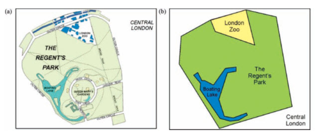
Fig. 19.1. (a) A topographic map showing the Regent’s Park in London; and (b) a topological map showing the location of the London zoo and the Boating Lake which lie inside the Regent’s Park in London .

(Source: Liu, and Mason, 2009)

19.2.7 Contiguity or Adjacency

Contiguity, a related concept, allows the determination of adjacency between features. Two features can be considered adjacent if they share a boundary. Hence, the polygon representing London Zoo can be considered adjacent to Regent’s Park.The from-node and to-node define an arc’s direction, so that the polygons onits left and right sides must also be known, left–right topology describes this relationship and therefore adjacency.

19.2.8 Extending the Vector Data Model

Topology allows us to define areas and to model three types of association, namely connectivity, area definition and adjacency (or contiguity), but we may still need to add further complexity to the features we wish to describe. For instance, a featuremay represent a composite of other features, so that a country could be modelled as the set of its counties, where the individual counties are also discrete and possibly geographically disparate features. Alternatively, a feature may change with time,and the historical tracking of the changes may be significant. For instance, a parcel of land might be subdivided and managed separately but the original shape, size and attribute information may also need to be retained. Other examples include naturally overlapping features of the same type, such as the territories or habitats of several species, or the marketing catchments of competing supermarkets, or surveys conducted in different years as part of an exploration program (as illustrated in Fig. 19.2). The ‘spaghetti’ model permits such area subdivisionand/or overlap but cannot describe the relationships between the features. Arc-node topology can allow overlaps only by creating a new feature representing the area of overlap, and can only describe a feature’s relationship with its subdivisions by recording that information in the attribute table. Several new vector structures have been developed by ESRI and incorporated into its ArcGIS technology. These support and enable complex relationships and are referred to as regions, sections, routes and events.

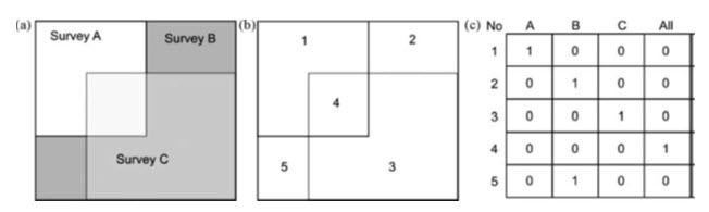
Fig. 19.2. (a) Map of the boundaries of three survey areas, carried out at different times. Notice that the areas overlap in some areas; this is permitted in ‘spaghetti’ data but not in arc-node structures; (b) the same survey maps after topological enforcement to create mutually exclusive polygonal areas; (c) the attribute table necessary to link the newly created polygons (1 to 5) to the original survey extents (A, B and C).

(Source: Modified after Bonham-Carter, 2002)

19.2.8.1 Regions

A region consists of a loose association of related polygons and allows the description of the relationships between them. A series of arcs and vertices construct a polygon and a series of polygon forms a region. The polygon comprising the region may be listed in any order. Point’s lines and polygon has a unique identifier. The polygons representing the features within the region are independent, they may overlap and they do not necessarily cover the entire area represented by the region. So overlapping survey areas in fig 19.2 could simply be associated within a survey region. Constructing overlapping regions is rather similar to constructing polygons; where regions overlap, they share a polygon in the same way that polygons share an arc where they meet, as shown in Fig. 19.3

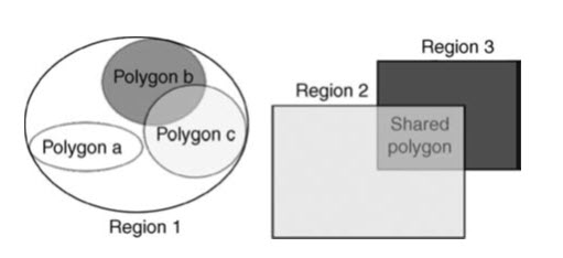
Fig. 19.3. Illustration of different types of region: associations of polygons and overlapping polygons which share a polygon.

(Source: Liu, and Mason, 2009)

19.2.8.2 Linear referencing

Routes, sections and events can be considered together since they tend not to exist on their own, and together they constitute a system of linear referencing as it is termed in ESRI’s ArcGIS. The constructed route defines a new path along an existing linear feature or series of features, as illustrated in Fig. 19.4.

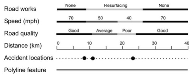
Fig. 19.4. Several routes representing different measures (linear and point events), created from and related to a pre-existing polyline feature representing, in this case, a road network. (Source: Liu, and Mason, 2009)

• ROUTE

A route may be circular, beginning and ending in the same place. Routes may be disconnected, such as one that passes through a tunnel and so is not visible at the surface. A further piece of information necessary for the description of a route is the unit of measurement along the route. This could be almost any quantity and for the example of a journey the measure could be time or distance.

• SECTION

A section describes particular portions of a route, such as a where road works are in progress on a motorway, where speed limits are in place on a road, or where a portion of a pipeline is currently undergoing maintenance. Again, starting and ending nodes of the section must be defined according to the particular measure along the route.

• EVENT

An event describes specific occurrences along a route, and events can be further subdivided into point and linear events. A point event describes the position of a point feature along a route, such as an accident on a section of motorway or a leak along a pipeline. The point event’s position is described by a measure of, for instance, distance along the route. A linear event describes the extent of a linear feature along a route, such as speed restrictions along a motorway, and is rather similar in function to a section. A linear event is identified by measures denoting the positions where the event begins and ends along the route.Route and event structures are of use in the description of application-specific entities such as seismic lines and shot-point positions. Since conventional vector structures cannot inherently describe the significance of discrete measurements along such structures. Along seismic lines the shot points are the significant units of measurement but they are not necessarily regularly spaced or numbered along that line, so they do not necessarily denote distance along it or any predictable quantity.

19.2.9 Representing surfaces

The vector data model provides several options for surface representation. Iso-lines (or contours), the triangulated irregular network, or TIN, and, Thiessen polygons (although less commonly used). Contours can only describe the surfaces from which they were generated and so do not readily facilitate the calculation of further surface parameters, such as slope angle, or aspect (the facing direction of that slope); both of these are important for any kind of ‘terrain’ or surface analysis. The techniques surrounding the calculation of contours are comprehensively covered in many other texts and so we will skirt around this issue here.

19.2.9.1 TIN Surface Model (Triangulated Irregular Network)

The TIN data model describes a 3D surface composed of a series of irregularly shaped and linked but non-overlapping triangles. The TIN is also sometimes referred to as the ‘irregular triangular mesh’ or ‘irregular triangular surface model’. The points which define the triangles can occur at any location, hence the irregular shapes. This method of surface description differs from the raster model in three ways. Firstly, it is irregular in contrast with the regular spacing of the raster grid; secondly, the TIN allows the density of point spacing (and hence triangles) to be higher in areas of greater surface complexity (and requires fewer points in areas of low surface complexity); and lastly it also incorporates the topological relationships between the triangles.

The process of Delaunay triangulation is used to connect the input points to construct the triangular network. The triangles are constructed and arranged so that no point lies inside the circumcircle of any triangle (Fig. 19.5). Delaunay triangulation maximizes the smallest of the internal angles and so tends to produce ‘fat’ rather than ‘thin’ triangles.

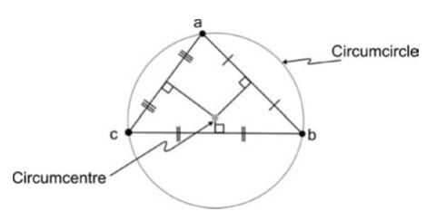
Fig. 19.5. The Delaunay triangle constructed from three points by derivation of the circumcircle and circumcentre; the position of the latter is given by the intersection of the perpendicular bisectors from the three edges of the triangle. (Source: Liu, and Mason, 2009)

As with all other vector structures, the basic components of the TIN model are the points or nodes, and these can be any set of mass points with which are stored values other than x, y and a unique identifying number, i.e. a z value in their attribute table. Nodes are connected to their nearest neighbours by edges, according to the Delaunay triangulation process.

The input mass points may be located anywhere.Of course the more carefully positioned they are, themore closely the model will represent the actual surface. TINs are sometimes generated from raster elevation models, in which case the points are located according to an algorithm that determines the sampling ratio necessary to describe the surface adequately. Well-placed mass points occur at the main changes in the shape of the surface, such as ridges, valley floors, or at the tops and bottoms of cliffs

TINs allow rapid display and manipulation but have some limitations. The detail with which the surface morphology is represented depends on the number and density of the mass points and so the number of triangles. So to represent a surface as well and as continuously as a raster grid, the point density would have to match or exceed the spatial resolution of the raster. Further, while TIN generation involves the automatic calculation of slope angle and aspect for each triangle, in the process of its generation, the calculation and representation of other surface morphological parameters, such as curvature, are rather more complex and generally best left in the realm of theraster. (Liu & Mason, 2009)

A) Advantage of Vector Data

• Data can be represented at its original resolution and form without generalization.

• Graphic output is usually more aesthetically pleasing (traditional cartographic representation).

• Accurate geographic location of data is maintained.

• Hard copy maps, is in vector form no data conversion is required.

(B) Disadvantage of Vector Data:

• The cell size determines the resolution at which the data is represented.

• It is especially difficult to adequately represent linear features depending on the cell resolution. Accordingly, network linkages are difficult to establish.

• Processing of associated attribute data may be cumbersome if large amounts of data exists. Raster maps inherently reflect only one attribute or characteristic for an area.

• Since most input data is in vector form, data must undergo vector-to-raster conversion. Besides increased processing requirements this may introducedata integrity concerns due to generalization and choice of inappropriate cell size.

• Most output maps from grid-cell systems do not conform to high-quality cartographic needs.

(http://bgis.sanbi.org/gis-primer/page_19.htm Accessed on 03.12.2012.)

Keywords: Data quantization and storage, Spatial variability, Spaghetti data, Unstructured or Vertex dictionary, Dual Independent Map Encoding (DIME), Arc-node Structure or “POLYVRT” (POLYgonconVeRTer) Contiguity or Adjacency, Triangulated Irregular Network.

References

• Liu, J.G., Mason, P.J., (2009). Essential Image Processing and GIS for Remote Sensing, UK.

• http://bgis.sanbi.org/gis-primer/page_19.htm Accessed on 03.12.2012.