
Site pages
Current course
Participants
General
Module 1: Introduction and Concepts of Remote Sensing
Module 2: Sensors, Platforms and Tracking System
Module 3: Fundamentals of Aerial Photography
Module 4: Digital Image Processing
Module 5: Microwave and Radar System
Module 6: Geographic Information Systems (GIS)
Module 7: Data Models and Structures
Module 8: Map Projections and Datum
Module 9: Operations on Spatial Data
Module 10: Fundamentals of Global Positioning System
Module 11: Applications of Remote Sensing for Eart...
Lesson 20 Data Structures
20.1 Introduction
The raster and vector methods of spatial data structure are two different approaches for modelling graphical information. Earlier the notion was that the raster and vector data structures were irreconcilable alternatives. However, now-a-days it is accepted that these two approaches have to be used in a synergetic manner for optimal results. Raster method requires huge computer memories to store and process image at the level of spatial resolution obtained by vector structures. Certain operations such as polygon intersection or spatial averaging presented enormous technical problems with the choice of raster methods that allowed easy spatial analysis but resulted in poor maps or vector methods that could provide database of manageable size and elegant graphics but in which spatial analysis was extremely difficult. The problem of raster or vector disappears once it is realised that both are valid methods for representing spatial data, and that both structures are inter-convertible. Conversion from vector to raster (rasterization) is the simplest. The reverse operation i.e. raster to vector (vectorization) is also well understood but is much more complex operation that is complicated by the need to reduce the number of coordinates in the resulting line by a process known as weeding. (http://nptel.iitm.ac.in/courses/Webcourse-contents/IIT-KANPUR/ModernSurveyingTech/lectureE_37/E_37_4.htm).
In this unit we will focus on the conversion of data structures from vector-to-raster (rasterization) as well as from raster-to-vector (vectorization). A little description of the various errors produced due to the conversion of data structure is also included in the end of the chapter.
20.1.1 Geo-data
As Geo-data we can define every dataset that has a spatial aspect or component. It can also be called as "spatial data", "geographic data", "geographic data sets" or "GIS data". The syllable "Geo" implies that the dataset has a spatial component that allows to geo-reference the described phenomena to a location or region on the earth.
20.1.2 Geo-data structure
As geo-data structure we can define the logical, internal data organization of our geographic information, the means of representing a real-life entity inside a geo-data model. Data structures should enable data storage and data management, as well as quick retrieval of the data. Unique identifier, links, relationships and dependencies help to build consistent and normalized data structures and enable links within the dataset or to external data sources.
20.1.3 Geo-data model
A geo-data model is an abstract, artificially created mapping of a part of the real world relevant to a geo-informatics project. The goal of geo-data modelling is to map the relevant conditions and processes in the real world to geo-data structure. A data model not only describes the content, properties and data structures, but also rules and relations between the entities of a data model. (https://geodata.ethz.ch/geovite/tutorials/L2GeodataStructuresAndDataModels/en/html/L2GeodataStructuresAndDataModels_glossary.html).
20.2 Conversion between Data Models and Structures
Spatial data can be represented in two formats, raster (grid cell) or vector (polygon). Raster data such as satellite images and scanned maps are comprised of numerically coded grid cells. Vector data are comprised of coded points, lines, and polygons. There are sometimes circumstances when conversion from raster to vector formats is necessary for display and/or analysis. Data may have been captured in raster form through scanning, for instance, but may be needed for analysis in vector form (e.g. elevation contours needed to generate a surface, from a scanned paper topographic map). Data may have been digitized in vector form but subsequently needed in raster form for input to some multi-criteria analysis. In such cases it is necessary to convert between models and some consideration is required as to the optimum method, according to the stored attributes or the final intended use of the product. Moreover, there are different types of vector and raster formats for data structures, which make it necessary to have intra format data conversion procedures. Thus there are four sets of conversion methods (Adam and Gangopadhyay, 2000):
(i) Raster to raster
(ii) Raster to vector
(iii) Vector to raster
(iv) Vector to vector
Most geographic information systems (GIS) now provide software for such a conversion. There are a number of processes which fall under this description and these are summarized in Table 20.1
Table 20.1 Summary of general conversions between feature types (points, lines and areas), in vector/raster form
|
Conversion type |
To point/pixel |
To line |
To polygon/area |
|
From point/pixel |
Grid or lattice creation |
Contouring, line scan conversion/filling |
Building topology, TIN, Thiessen polygons/ interpolation, dilation |
|
From line |
Vector intersection, line splitting |
Generalizing, smoothing, thinning |
Buffer generation, dilation |
|
From polygon/area |
Centre point derivation, vector intersection |
Area collapse, skeletonization, erosion, thinning |
Clipping, subdivision, merging |
(Source: Liu and Mason, 2009)
20.3 Different uses of the Data in GIS
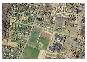
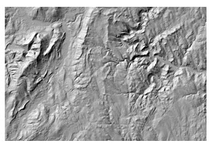
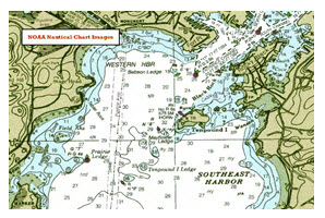
Since raster data refers directly to spatial extensions instead of lines or points, as it is in vector data, it is difficult to overlay with other raster data information, that's why it is often used as background information. The difference between typical GIS raster data sets and vector data sets are illustrated in following section:
Typical GIS raster data sets
|
(a) Orthophoto |
(b) Relief |
|
(c) Crop evapotranspiration |
(d) Nautical chart |
Fig. 20.1. Examples of typical GIS raster dataset.
(Source: https://geodata.ethz.ch/geovite/tutorials/L2GeodataStructuresAndDataModels/en/html/unit_u4VecVsRas.html; accessed on Dec 02, 2012)
Advantages of Raster Data Structures
Simple data structure
Easy to generate (e.g. from remote sensing or scan-digitizing)
Easy workflows and analysis
Technology is cheap and is being energetically developed
Overlay and limitation of mapped data with remotely sensed data is easy
Various kinds of analytical (spatial) operations are easy
Simulation is very easy as each spatial unit has the same shape and size
Same set of grid cells are used for several variables
Simple when doing your own programming
Disadvantages of Raster Data Structures
Non-adaptive data structure
Tends to generate huge files, depending on resolution
Cell arrangement is usually random and does not respect natural borders
Limited interactivity and more primitive analysis algorithms
Errors in evaluating perimeter of shape
Topology or network linkages are difficult to establish
Geometric transformations are difficult to handle
Use of large cells to reduce data volumes result into loss of information
Usage Scenarios of Raster Data Structures
Photos
Photogrammetry and remote sensing
Scanned images of maps
Terrain modelling
Landcover analysis
Hydrologic modelling and analysis
General GIS surface modelling and analysis for continuous surfaces
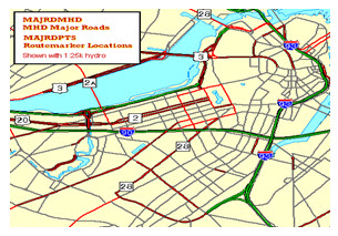
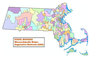
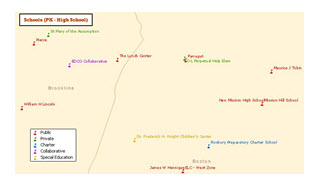
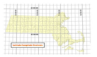
Typical GIS vector data sets
|
(a) Highway
|
(b) House districts |
|
(c) Schools
|
(d) Latitude/longitude grid |
Fig. 20.2. Examples of typical GIS vector dataset.
(Source: Liu and Mason, 2009)
Advantages of Vector Data Structures
Small amount of data
Logical data structure
Attributes are combined with objects
Preserves quality after interactivity (e.g. scaling)
More sophisticated in spatial analysis
Topology described with network linkages
Retrieval, updating and generalization of graphics and attributes are possible
Widely used to described administrative zones
(http://nptel.iitm.ac.in/courses/Webcourse-contents/IIT-KANPUR/ModernSurveyingTech/lectureE_37/E_37_4.htm)
Disadvantages of Vector Data Structures
Complex data structure
Continuous data is not represented effectively
Spatial variability is not implicitly represented
Spatial analysis and filtering within polygons is impossible
Needs a lot of manual editing to get good quality
It always introduces hard boundaries
Simulation is difficult as each unit has different topological form
Overlaying of several polygon maps or polygon and raster maps is difficult
Display and plotting can be expensive
(http://nptel.iitm.ac.in/courses/Webcourse-contents/IIT-KANPUR/ModernSurveyingTech/lectureE_37/E_37_4.htm)
Usage Scenarios of Vector Data Structures
CAD, technical drawings
Street or river networks, cadastral maps
Network analysis
Cartography
(http://nptel.iitm.ac.in/courses/Webcourse-contents/IIT-KANPUR/ModernSurveyingTech/lectureE_37/E_37_4.htm)
20.4 Intra-Format Conversion
Raster to raster and vector to vector data conversions are the types of intra-format conversion methods. Raster formats differ in the way they are stored. Three commonly used storage strategies for data in raster formats are band sequential (BSQ), band interleaved by pixels (BIP) and band interleaved by lines (BIL). The purpose of all these strategies is to efficiently stored raster structure data for different thematic layers. For example, a given geographic study area may have three thematic data layers: land elevation, rainfall and slope. Each of these layers will be stored in a separate raster structure with the same resolution. These individual raster structures can be stored in different files, which is called the BSQ strategy; or the pixels (raster cells) can be stored sequentially with all data value stored after each pixels, which is the BIL strategy. Conversion between raster formats requires reorganization of the raster cells and their corresponding data values, which is a relatively simple operation as compare to inter format conversion.
Vector to vector conversion is necessitated due to the usage of different types of vector formats. Data structures in vector formats can be classified into two primary categories. In the first category is the whole polygon method in which the polygons are stored in terms of the coordinates of the vertices. In this method the nodes and the arc are implicitly represented. In contrast other methods, including DIME (Dual Independent Map Encoding), arc-node and relational structures are variation of the arc node structure, where nodes arcs and polygons are stored in the tabular formats.
20.5 Inter-Format Conversion
Inter format conversion consists of two types (Adam and Gangopadhyay, 2000):
(a) Vector to raster
(b) Raster to vector
20.5.1 Vector to raster conversion (rasterization)
These processes begin with the identification of pixels that approximate significant points, and then pixels representing lines are found to connect those points. The locations of features are precisely defined within the vector coordinate space but the raster version can only approximate the original locations, so the level of approximation depends on the spatial resolution of the raster. The finer the resolution, the more closely the raster will represent the vector feature. Many GIS programs require a blank raster grid as a starting point for these vector–raster conversions where, for instance, every pixel value is ‘0’ or has a null or no data value. During the conversion, any pixels that correspond to vector features are then ‘turned on’: their values are assigned a numerical value to represent the vector feature.
20.5.1.1 Point to raster
For conversions between vector points and a discrete raster representation of the point data, there are several ways to assign a point’s value to each pixel (as shown in Fig 20.3). The first is to record the value of the unique identifier from each vector point. In this case, when more than one vector feature lies within the area of a single pixel, there is a further option to accept the value of either the first or the last point encountered since there may be more than one within the area of the pixel. Another option is to record a value representing merely the presence of a point or points. The third choice is to record the frequency of points found within a pixel. The fourth is to record the sum of the unique identifying numbers of all vector points that fall with the area of the output pixel. The last is to record the highest priority value according to the range of values encountered.
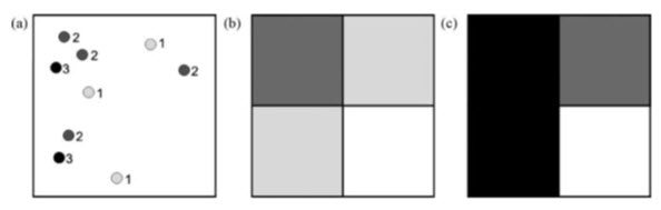
Fig. 20.3. (a) Input vector point map (showing attribute values). (b) and (c) Two different resulting raster versions based on a most frequently occurring value rule (if there is no dominantly occurring value, then the lowest value is used) (b), and a highest priority class rule (where the attribute values 1–3 are used to denote increasing priority) (c).
(Source: Liu and Mason, 2009)
Point, line and polygon features can be converted to a raster using either textual or numerical attribute values. Only numbers are stored in the raster file– numbers in a value range which dictates how the raster data are quantized, as byte or integer data for instance. So if text fields are needed to describe the information in the output raster, an attribute table must be used to relate each unique raster DN to its text descriptor. When pixels do not encounter a point, they are usually assigned a null (No Data) or zero value. The last is to record the highest priority value according to the range of values encountered.
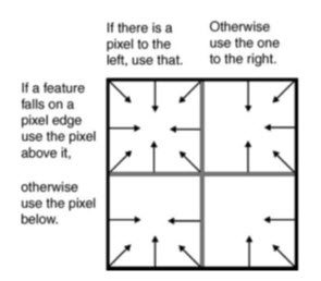
Fig. 20.4. Boundary inclusion rules applied when a feature falls exactly on a pixel boundary. Arrows indicate the directional assignment of attribute values. (Source: Modified after ESRI’s ArcGIS online knowledge base)
The above rules decide the value assigned to the pixel but further rules are required when points fall exactly on the boundary between pixels. These are used to determine which pixel will be assigned the appropriate point value. The scheme used within ESRI’s ArcGIS is illustrated in Fig 20.4, in which a kind of kernel and associated logical rules provide consistency by selecting the edge and direction to which the value will be assigned.
Point to raster area conversions also includes conversion to the continuous raster model. This category generally implies interpolation or gridding, of which there are many different types.
20.5.1.2 Polyline to raster
A typical line rasterizing algorithm first finds a set of pixels that approximate the locations of nodes. Then lines joining these nodes are approximated by adding new pixels from one node to the next one and so on until the line is complete. As with points, the value assigned to each pixel when a line intersects it is determined by a series of rules. If intersected by more than one feature, the cell can be assigned the value of the first line it encounters, or merely the presence of a line (as with point conversions above), or of the line feature with the maximum length, or of the feature with the maximum combined length (if more than one feature with the same feature ID cross it), or of the feature that is given a higher priority feature ID (as shown in Fig 20.5).

Fig. 20.5. (a) Input vector line map. (b) to (d) Three different resulting raster versions based on a maximum length rule (or presence/absence rule) (b), maximum combined length rule (c) and a highest priority class rule (d) where the numbers indicate the priority attribute values.
(Source: Liu and Mason, 2009)
Again, pixels which are not intersected by a line are assigned a null or No Data value. Should the feature fall exactly on a pixel boundary, the same rules are applied to determine which pixel is assigned the line feature value, as illustrated in Fig 20.4.
The rasterizing process of a linear object initially produces a jagged line, of differing thickness along its length, and this effect is referred to as aliasing. This is visually unappealing and therefore undesirable but it can be corrected by anti-aliasing techniques such as smoothing. When rasterizing a line or arc the objective is to approximate its shape as closely as possible, but, of course, the spatial resolution of the output raster has a significant effect on this.
20.5.1.3 Polygon to raster
The procedures used in rasterizing polygons are sometimes referred to as ‘polygon scan conversion’ algorithms. These processes begin with the establishment of pixel representations of points and lines that define the outline of the polygon. Once the outline is found, interior pixels are identified according to inclusion criteria; these determine which pixels that are close to the polygon’s edge should be included and which ones should be rejected. Then the pixels inside the polygon are assigned the polygon’s identifying or attribute value. This value will be found from the pixel that intersects the polygon centre. The inclusion criteria in this process may be one of the following, whose effects are illustrated in Fig 20.6:
a) Central point rasterizing, where the pixel is assigned the value of the feature which lies at its centre.
b) Dominant unit or largest share rasterizing, where a pixel is assigned the value of the feature (or features) that occupies the largest proportion of that pixel.
c) Most significant class rasterizing, where priority can be given to a certain value or type of feature, such that if it is encountered anywhere within the area of a pixel, the pixel is assigned its value.
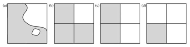
Fig. 20.6. (a) Input vector polygons map. (b) to (d) Three different resulting raster versions based on a dominant share rule (b), a central point rule (c) and a most significant class rule (d). (Source: Liu and Mason, 2009)
When viewed in detail (as in Figures 20.3, 20.5 and 20.6) it can be seen that the inclusion criteria have quite different effects on the form of the raster version of the input vector feature. Again, if the polygon feature’s edge falls exactly on a pixel edge, special boundary rules are applied to determine which pixel is assigned the line feature value, as illustrated in Fig 20.4.
20.5.2 Raster to vector conversion (vectorization)
20.5.2.1 Raster to point
All non-zero cells are considered points and will become vector points with their identifiers equal to the DN value of the pixel. The input image should contain zeros except for the cells that are converted to be points. The x, y position of the point is determined by the output point coordinates of the pixel centroid.
20.5.2.2 Raster to polyline
This process essentially traces the positions of any non-zero or non-null raster pixels to produce a vector polyline feature, summarized in Fig 20.7.
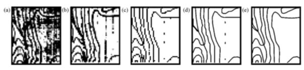
Fig. 20.7. Illustration of polygon scan vectorization procedures: (a) image improvement by conversion to binary (bi-level) image; (b) thinning or skeletonization process to reduce thickness of features to a single line of pixels; (c) vectorized lines representing complex areas; (d) collapsed but still including spurious line segments; and (e) the lines are smoothed or ‘generalized’ to correct the pixelated appearance and line segments removed. (Source: Liu and Mason, 2009)
One general requirement is that all the other pixel values should be zero or a constant value. Not surprisingly, the input cell size dictates the precision with which the output vertices are located. The higher the spatial resolution of the input raster, the more precisely located the vertices will be. The procedure is not simple and generally involves several steps and is summarized as follows:
Filling: The image is first converted from a greyscale to a binary raster (through reclassification or thresholding), then any gaps in the features are filled by dilation.
Thinning: The line features are then thinned, skeletonized or eroded, i.e. the edge pixels are removed in order to reduce the line features to an array or line of single but connected pixels.
Vectorizing: The vertices are then created and defined at the centroids of pixels representing nodes, that is where there is a change in orientation of the feature. The lines are produced from any connected chains of pixels that have identical DN value. The resultant lines pass through the pixel centres. During this process, many small and superfluous vertices are often created and these must be removed. The vectors produced may also be complex and represent area instead of a true linear feature.
Collapsing: Complex features are then simplified by reducing the initial number of nodes, lines and polygons and, ideally, collapsing them to their centre lines. One commonly adopted method is that proposed by Douglas and Peucker (1974), which has subsequently been used and modified by many other authors.
Smoothing: The previous steps tend to create a jagged, pixelated line, producing an appearance which is rather unattractive to the eye; the vector features are then smoothed or generalized, to smooth this appearance and to remove unnecessary vertices. This smoothing may be achieved by reducing the number of vertices, or using an averaging process (e.g. a three- or five-point moving average).
20.5.2.3 Raster to polygon
This is the process of vectorizing areas or regions from a raster. Unless the raster areas are all entirely discrete and have no shared boundaries, it is likely that the result will be quite complex. Commonly, therefore, this process leads to the generation of both a line and a polygon file, in addition to a point file representing the centres of the output polygons The polygon features are constructed from groups of connected pixels whose values are the same. The process begins by determining the intersection points of the area boundaries and then follows this by generating lines at either external pixel centroids or the boundaries. A background polygon is also generated; otherwise any isolated polygons produced will float in space. Again, such vectorization procedures from raster images are usually followed by a smoothing or generalization procedure, to correct the ‘pixelated’ appearance of the output vectors. There are now a great many software suites available which provide a wealth of tools to perform these raster–vector conversions, some of which are proprietary and some ‘shareware’, such as MATLAB (MathWorks), AutoCAD (Autodesk), R2V (developed by Able Software Corp.), Illustrator, Freehand, etc.
20.6 Errors in Data Conversion
During vector to raster conversion both the size of the raster and the method of rasterization used have important implications for positional error and, in some cases, attribute uncertainty. The smaller the cell size the greater the precision of the resulting data. Finer raster sizes can trace the path of a line more precisely and therefore help to reduce classification error- a form of attribute error. Positional and attribute errors as a result of generalization are seen as classification error in cells along the vector polygon boundary. This is seen visually as the ‘stepped’ appearance of the raster version when compared with the vector original (Fig 20.8).
The conversion of data from raster to vector format is largely a question of geometric conversion; however certain topological ambiguities can occur- such as where different coded raster cells join at corner as in Fig 20.9. In this it is impossible to say, without returning to the original source data, whether the vector polygon should join. Where vector maps have been derived from raster data, conversion may result in a stepped appearance in the output map. This can be reduced, to some extent by line smoothing algorithms but these makes certain assumptions about topological relationships and detail that may not be present in the raster source data. (Heywood et al., 2010)
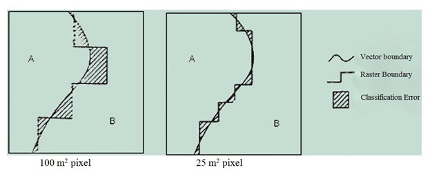
Fig. 20.8. Effect of size of raster cell (resolution) on representation of a feature. (Source: http://nptel.iitm.ac.in/courses/Webcourse-contents/IIT-KANPUR/ModernSurveyingTech/lectureE_40/E_40_3.htm)
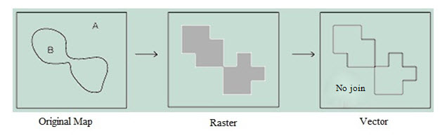
Fig. 20.9. Topological ambiguities. (Source: http://nptel.iitm.ac.in/courses/Webcourse-contents/IIT-KANPUR/ModernSurveyingTech/lectureE_40/E_40_3.htm)
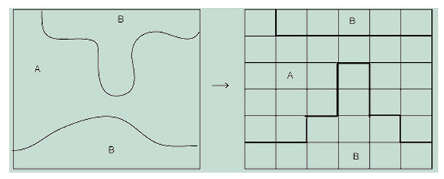
Fig. 20.10. Loss of connectivity and creation of false connectivity. (Source: http://nptel.iitm.ac.in/courses/Webcourse-contents/IIT-KANPUR/ModernSurveyingTech/lectureE_40/E_40_3.htm)
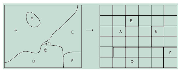
Fig. 20.11. Loss of information (What happened to ‘C’ ?). (Source: http://nptel.iitm.ac.in/courses/Webcourse-contents/IIT-KANPUR/ModernSurveyingTech/lectureE_40/E_40_3.htm)
Keywords: Geo-data structure, Geo-data model, Intra-format conversion, Inter-format conversion, rasterization, vectorization, Thinning, Collapsing.
Reference
Liu, J.,G. and Mason, P., J., 2009, Essential Image Processing and GIS for Remote Sensing, John Wiley & Sons Ltd., pp. 157-161.
Adam, N.R. and Gangopadhyay, A., 2000, Database Issues in Geographic Information Systems, Kluwer Academic Publishers, Massachusetts (USA), pp. 43-44.
Heywood, I., Cornelius, S. and Carver, S., 2010, An Introduction to Geographical Information Systems, Dorling Kindersley (India) Pvt. Ltd, pp. 313-315.
https://geodata.ethz.ch/geovite/tutorials/L2GeodataStructuresAndDataModels/en/html/unit_u4VecVsRas.html; accessed on Dec 02, 2012.
https://geodata.ethz.ch/geovite/tutorials/L2GeodataStructuresAndDataModels/en/html/L2GeodataStructuresAndDataModels_glossary.html; accessed on Dec 02, 2012.
https://geodata.ethz.ch/geovite/tutorials/L2GeodataStructuresAndDataModels/en/html/unit_u2Raster.html; accessed on Dec 02, 2012.
https://geodata.ethz.ch/geovite/tutorials/L2GeodataStructuresAndDataModels/en/html/unit_u3Vector.html; accessed on Dec 02, 2012.
http://nptel.iitm.ac.in/courses/Webcourse-contents/IIT-KANPUR/ModernSurveyingTech/lecture E_37/E_37_4.htm; accessed on Dec 02, 2012.
http://nptel.iitm.ac.in/courses/Webcourse-contents/IIT-KANPUR/ModernSurveyingTech/lectureE_40/E_40_3.htm; accessed on Dec 02, 2012.
Last modified: Friday, 31 January 2014, 5:51 AM