CAD/CAM Machine Drawing and Computer Graphics 3(1+2)

LESSON 12. Analytical and synthetic approaches, parametric and implicit equations

12.2.Analytical and synthetic approaches

Curves are used to draw a wireframe model, which consists of points and curves; the curves are utilized to generate surfaces by performing parametric transformations on them. A curve can be as simple as a line or as complex as a B-spline. In general, curves can be classified as follows:

Analytical Curves: This type of curve can be represented by a simple mathematical equation, such as, a circle or an ellipse. They have a fixed form and cannot be modified to achieve a shape that violates the mathematical equations.

Interpolated curves: An interpolated curve is drawn by interpolating the given data points

and has a fixed form, dictated by the given data points. These curves have some limited flexibility in shape creation, dictated by the data points.

Approximated Curves: These curves provide the most flexibility in drawing curves of very

complex shapes. The model of a curved automobile fender can be easily created with the help

of approximated curves and surfaces. In general, sweeping a curve along or around an axis creates a surface, and the generated surface will be of the same type as the generating curve, e.g., a fixed form curve will generate a fixed form surface.

12.3.Parametric and implicit equations

In mathematics, parametric equation is a method of defining a relation using parameters The mathematical representation of a curve can be classified as either parametric or nonparametric (natural). A non-parametric equation has the form,

y = c1 + c2 x + c3 x² + c4 x³          non-parametric equation

This is an example of an explicit non-parametric curve form.

In this equation, there is a unique single value of the dependent variable for each value of the independent variable. The implicit non-parametric form of an equation is,

(x – xc)² + (y – yc)² = r²                 Implicit non-parametric equation

In this equation, no distinction is made between the dependent and the independent variables.

This equation gives the flexibility to generate any curve form depending on our requirement in computer graphics.

Parametric Equations

Parametric equations describe the dependent and independent variables in terms of a parameter. The equation can be converted to a non-parametric form, by eliminating the dependent and independent variables from the equation. Parametric equations allow great versatility in constructing space curves that are multi-valued and easily manipulated. Parametric curves can be defined in a constrained period (0 ≤ t ≤ 1); since curves are usually bounded in computer graphics, this characteristic is of considerable importance. Therefore, parametric form is the most common form of curve representation in geometric modeling. Examples of parametric and non-parametric equations follow.

Let us study a straight line in a plane as a simple first example.

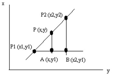
The triangles P1,A,P and P1,B,P2 are similar and we can set up the following:

and find for example y expressed by coordinates for the two known points and x.

As an alternative we could set up a parametric equation for the line. Parametric means that the expression contains a parameter, t, that changes when we run along the line. For a line in the plane we get two parametric expressions, one for x and one for y. Since we have a line, both are linear.

      P=P1+t·(P2-P1)

      x(t)=x1+(x2-x1)·t

      y(t)=y1+(y2-y1)·t

We see that x(0)=x1 and y(0)=y1, and x(1)=x2 and y(1)=y2. Since the expressions are linear we know that when t runs from 0 to 1, x and y runs from P1 to P2.

A parametric form gives control over the length of the line, not only the line direction.

Even this simple example can be useful in some situations. If we are going to carry out an animation that moves in a straight line, we can control the animation with small t-steps. We control speed by varying the t-steps. More compound movements can be controlled by a sequence of linear movements, if we don't come up with something more clever.

An extension to include lines in space is simple. If we know the end points: P1(x1,y1,z1) and P2(x2,y2,z2), we get:

      P=P1+t·(P2-P1)

       x(t)=x1+(x2-x1)·t

      y(t)=y1+(y2-y1)·t

      z(t)=z1+(z2-z1)·t

(courtesy: www.it.hiof.no/~borres.com

Consider the unit circle which is described by the ordinary (Cartesian) equation

  Implicit form

This equation can be parametrized as well, giving

With the Cartesian equation it is easier to check whether a point lies on the circle or not. With the parametric version it is easier to obtain points on a plot.

Where, ‘t’ is the parameter.

CAD programs prefer a parametric equation for generating a curve. Parametric equations are

converted into matrix equations to facilitate a computer solution, and then varying a parameter from 0 to 1 creates the points or curves.