Mechanics of Tillage and Traction 3(2+1)

LESSON 14. Dimensional Analysis

14.2. Dimensions

The various physical quantities used by the engineers and the scientists, to describe a given phenomenon can be described by a set of quantities which are in a sense independent of each other. Thee quantities are known as fundamental or primary quantities. The primary quantities are mass, length, time and temperature, designated by the letters M, L, T, and θ  respectively. All other quantities such as area, volume, velocity, acceleration, force, energy, power etc., are termed as derived quantities or secondary quantities, because they can be expressed in terms of the primary quantities. The expression for a derived quantity in terms of the primary quantities is called the dimensions of the physical quantity. For example the dimension of force can be expressed as

[Force] = [ Mass X Acceleration]

Since, \[\left[ {Acceleration} \right]={L \over {{T^2}}}\]

\[\left[ {Force} \right]={{ML} \over {{T^2}}}=\left[ {ML{T^{ - 2}}} \right]\]

The rectangular bracket signifies that the dimensions of the quantity are being considered.

14.3. Dimensional Homogeneity

An equation will be said to be dimensionally homogeneous if the form of the equation does not depend on the fundamental units of measurement. In other words, an equation is said to be dimensionally homogenous, if the dimensions of the terms on its left hand side are same as dimensions of the terms on its right hand side. For example, the equation for the period of oscillation of a simple pendulum \[\left( {T = 2\sqrt {{L \over g}} } \right)\]  is valid whether length is measured in feet, meters, or miles, and whether time is measured in minutes, days, or seconds. Therefore, by definition, the equation is dimensionally homogeneous. If the value g = 32.2 ft/sec² is substituted in the equation, there results \[T=1.11\sqrt L\] . This equation is correct for pendulums on the earth, but it is no longer homogenous, since the factor 1.11 applies only if length is measured in feet and time is measured in seconds. It might be argued that the factor 1.11 itself has the dimension [L^-1/2T]. However, dimensions must not be assigned to numbers, for then any equation could be regarded as dimensionally homogenous.

It can be deduced from the above definition of dimensional homogeneity that an equation of the form x = a + b + c + …… is dimensionally homogeneous if, and only if, the variables x, a, b, c, …… all have the same dimensions. If a derived equation contains a sum or a difference of two terms that have different dimensions, a mistake has been made. This principle may be applied to differential equations and integral equations, as well as to algebraic equations. It should not be assumed, however, that an empirical equation is necessarily dimensionally homogeneous.

Every measurement has two characteristics: quantitative and qualitative. Dimensional analysis deals with the qualitative aspects of measurements. Qualitative aspects of measurements are expressed in terms of either primary or secondary units. The primary units are internationally accepted reference quantities in terms of which other quantities are specified (Skoglund, 1967). For example kg, m, s, and K are respectively the primary units of mass, length, time, and temperature in SI units. The derived or secondary units are expressed in terms of primary units based on mathematical relationships (Murphy, 1950). Thus speed, which is distance/time has the unit m/s.

Fundamental or basic quantities are a set of quantities that are chosen to represent other quantities based on convenience. Fundamental quantities may not be the same as primary quantities. Often force is chosen as a fundamental quantity in engineering, although it is not a primary quantity. The dimensions of these basic quantities are used in obtaining the dimensions of other quantities. Thus, if force (F), length (L), time (T), and temperature (θ) are used as fundamental quantities, then mass will have the following dimensions:

From Newton's second law:

force                = mass × acceleration ------------------------------------ (1.1)

Acceleration     =  \[{{{d^2}x} \over {d{t^2}}}\] ------------------------------------ (1.2)                  

where x is displacement, and t is time. From equations 1.1 and 1.2, mass is given by:

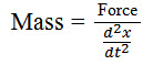             ------------------------------------ (1.3)

or, in terms of dimensions:

Here, force, length, time, and temperature are fundamental quantities. The power of dimensional analysis resides in its ability to classify equations, convert equations from one system of units to another, develop prediction equations, reduce the number of variables to be investigated in an experiment, and provide the basis for the theory of similitude (Murphy, 1950). Soil dynamics as a discipline has extensively benefited from these powerful features of dimensional analysis. This technique has been widely used during the1960s and 1970s to develop prediction equations, reduce the number of variables to be investigated, and conduct model studies.

Buckingham pi theorem:

Reduction in the number of variables

The Buckingham Pi theorem states that the number of Pi terms (s) required to express a relationship between variables is equal to the number of variables involved in the process (n) minus the number of dimensions (b) required to express those variables (Murphy, 1950; Palacios, 1964), i.e.:

s = n - b                                                                       (17)

Thus, in our example of a vertical wide blade operating in a cohesionless soil, we have five variables (cf. eq. 10) and two dimensions, resulting in three Pi terms. This theorem is particularly helpful in designing experiments, since it allows us to reduce the number of variables to be investigated, thus reducing the time required, complexity, and cost of conducting the experiments.

Form of Prediction Equations

The next task in developing the prediction equation is to determine the form of the prediction equation, e.g., whether equation 16 is the product or the sum of two component functions, f1(d/w) and f2(φ):

\[{D \over {{\rm{\gamma }}{{\rm{w}}^3}}}=Cf1\left( {{d \over w}} \right)f2\left( {\rm{\varphi }} \right){\rm{or}}{D \over {{\rm{\gamma }}{{\rm{w}}^3}}}=f1\left( {{d \over w}} \right) + f2\left( {\rm{\varphi }} \right)\]                   (18)

To address this issue, let us consider a general process that involves three Pi terms (π1, π2, π3), i.e., π1 = Φ(π2,π3).

The minimum number of tests necessary to determine the form of the prediction equation and verify that the form is Correct, is (2m - 3) for a process that involves m Pi terms (Murphy, 1950). Of these (2m - 3) tests, (m - 1) tests are necessary to determine the component equations, and the other (m - 2) tests are necessary to verify the form of the general response function. For the case when there are only three Pi terms, we need three tests to determine the form of the prediction equation. One of these tests can be conducted while keeping π3 constant at \[\bar \pi\]3(the bar is used to denote constant values). This test provides the component equation: f1(π2), i.e.,

Φ(π2, \[\bar \pi\]3) = π1\[\bar 3\] .

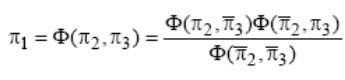
Similarly, component equation f2(π3), i.e., Φ(\[\bar \pi\]2, π3) = π1\[\bar 2\] , is obtained by conducting a second set of experiments while holding π2 constant at \[\bar \pi\]2 . Referring to figure 1, if the two component equations multiply to produce the prediction equation, then we have

where constant C can be shown to 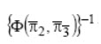 be Therefore, the form of the prediction equation is:

                       

To verify if the form of this equation is correct, a third test should be conducted by holding either π2 or π3 at some other level. Let us say that π3 is held at \[\bar \pi\]3 . Then the requirement for the prediction equation to be a product of two component equations is (Murphy, 1950):

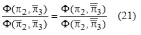
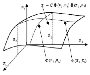
Figure 1. Graph of a prediction equation containing three π terms derived as a product of component equations.

A similar technique can be applied if the component equations are added to produce the prediction equation. Most soil dynamics problems involve more than three Pi terms. What happens if there are m Pi terms? Boyd (1966) outlined a procedure for determining complicated prediction equations. For example, if m = 5, then a total of seven (2m - 3) tests are necessary to develop the prediction equation and verify it. Of these seven tests, four tests (i.e., m - 1) are necessary to develop component equations. The other three tests (i.e., m - 2) are used for verifying the form of the prediction equation. These three equations lead to three conditions rather than just one, as shown in equation 21for a three-parameter case. Because of experimental error, these conditions are seldom exactly equal and a better approach is necessary to validate the form of the prediction. Shafii et al. (1996) proposed an alternate technique that can verify the form of the prediction equation using a rigorous statistical approach. Their approach is summarized below:

1. Conduct (m - 1) sets of tests holding all but one Pi term (πj) constant to determine the component equation f(πj) as:

f(πj) = Φ(π2, π3,...π j ,...πm) , for j = 2, 3, 4, ..., m                  (22)

2. If component equations multiply to yield the prediction equation, then it is expected to be of the form:

π1 = C Φ(π2 , π3,...π j ,...πm) Φ(π2, π3,...π j ,...πm) Φ(π2, π3,...π j ,...πm) Φ(π2, π3,..π j ,...πm) (23)

3. Estimate constant C from experimental data as:

                       

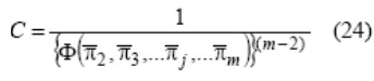
4. Obtain n additional data points corresponding to the values of the independent Pi terms (i.e., πj, j = 2, 3, ..., m) such that the values of πj fall within the range of interest for each of the Pi terms [i.e., (πj)min < πj < (πj)max]. Let these data be represented as:

{(π1k, π2k, π3k, ..., πjk, ..., πmk), k = 1, 2, 3, ..., n} (25)

5. Predict π1 corresponding to {(π2k, π3k, ..., πjk ..., πmk), k = 1, 2, 3, ..., n} using equations 23 and 24. Let these n estimated data points be represented by {( pπ1k ), k = 1, 2, 3, ..., n}.

6. Conduct a simple linear regression between π1k and pπ1k . If the form of the prediction equation is correct, then the slope of the regression equation should be close to 1.0 and the intercept should be almost zero. Moreover, the coefficient of determination (r2) should be close to 1.

APPLICATION OF DIMENSIONAL ANALYSIS AND SIMILITUDE METHODOLOGY TO SOIL-MACHINE SYSTEMS