Minor Irrigation & Command Area Development 3(2+1)

LESSON 22. METHODOLOGY TO WORKOUT WATER PRODUCTIVITY

22.1. Hypothetical model for all irrigation system

By and  large  the  term  model  refers  to  the  simplified representation of  a  system.  The functioning of a  system is so designed that the input parameters fed in to the system are processed  with  appropriate  mathematical  formulae  or  expressions  or  relations  with  or without constrains or ranges of applications, resulting in the output parameters designed. By the same token, water productivity either physical or economical is the system output for which the input parameters and the processes of manipulation have to be enumerated. The hypothetical or unique water productivity model can be developed by scrupulously following the procedures outlined herein.

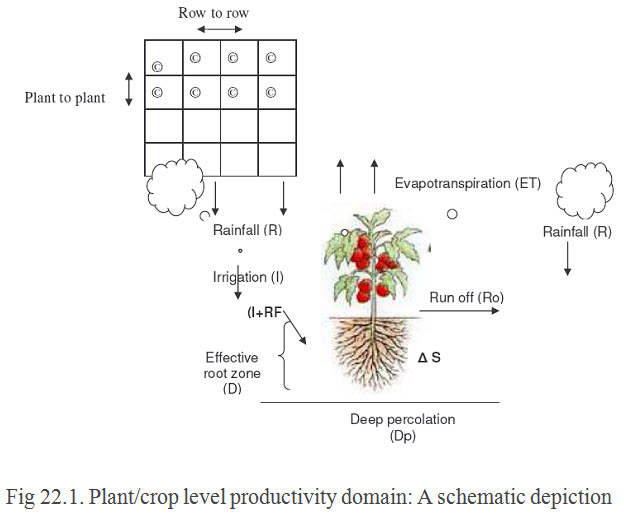
22.2. Plant/crop scale water productivity (WP(p)):

Here, the effective root zone of the plant/crop is the reference or datum over which the crop consumptive use exclusive of the inevitable gravitational irrigation system losses (seepage, run-off and deep percolation) is considered as the input for the single plant/crop output. In case of using micro-irrigation systems (Drip or Sprinkler) these losses are reduce to zero and the root zone gets exact replenishment through irrigation to meet the soil moisture deficit. The physiological processes such as photosynthesis, nutrient uptake and water stresses also contribute over productivity. Technically,

Total consumptive use (CU), cm = (total number of irrigation) *

(design depth of irrigation, cm)

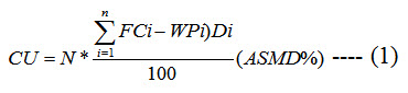
Where,

Di = Layer thickness of ith layer of the effective root zone, cm

FCi  = Field capacity moisture content (% vol.) of the ith layer

WPi  = Wilting point moisture content (% vol.) of the ith layer

ASMD = Allowable Soil Moisture Depletion, % (Taken as 50%)

i = 1,2,3…..n= no. of soil layers in the effective root zone depth

N = total number of irrigation

Then, water productivity on a plant/crop scale WP (p) = Y/CU and the water use efficiency becomes WUE (p) = WP (p)/A, where ‘A’ is the effective area commanded by the plant. In accordance with the crop-crop spacing (Sc) and the row-row spacing (Sr), A = Sc*Sr. The unit of WP(p) can be Kg yield per Kg of water consumed or cm of water consumed and that of WUE(p) can be Kg yield per cm of water consumed per square metre crop area.

The above equation holds good for a fully non-rainy season in which the consumptive use requirements are met only by irrigation. However, if rainfall occurs, then corrections should be made for including the effective rainfall as part of consumptive use. Generally, the term ‘effective rainfall’ in the context of agriculture is construed as that proportion of rainfall directly going to  replenish the soil moisture deficit till field capacity of the effective root zone is reached. After reaching field capacity moisture level, any addition of rainfall will be drained down beyond the effective root zone as deep percolation loss of water or the ineffective rainfall. During the rainfall periods, the frequency or the interval of applying the design depth of irrigation gets widened. The difference between total  consumptive use requirement  and  the  contribution  from  effective  rainfall  is  reckoned  as  the  isolated contribution from irrigation only. Technically,

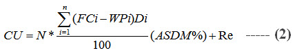
Where,

FC = Mean Field capacity moisture content of the effective root zone, % EM = Mean existing moisture content of the effective root zone, %

As = mean apparent specific gravity of the effective root zone,

D = Effective root zone depth, cm

R = incident rainfall, cm and

Re = effective rainfall, cm

Format 1. Plant/crop level water productivity

Crop

Effective root zone depth (D)   :  cm

Spacing                                  :  m  x  m

Plant grid area (A)                   :  m2

Soil                                        :

Average field capacity (FC)      :         %

Average wilting point (WP)      :         %

Average Apparent Specific Gravity   :

Allowable soil moisture depletion :   %

Runoff is assumed as Zero

Design depth of irrigation (d), cm = 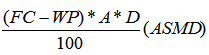 =  cm of water

No. of irrigation (N)       :  

Rainfall(R)                            :  cm

Effective Rainfall (Re)           :   cm

Soil profile moisture storage changes (S):  cm

 S= TPMCb - TPMCe

TPMCb = Total profile moisture content at the beginning of sowing, cm

TPMCe = Total profile moisture content at the end of harvest, cm

22.3. Field/Farm scale water productivity (WP (f)):

At a field scale, processes of interest are different: nutrient application, water conserving tillage practices, field bunding, puddling of paddy fields etc. Water enters the field domain by direct rainfall, subsurface flows and irrigation from a source of storage. Rainfall alone is considered in case of rain fed agriculture. A field or farm scale water productivity (WP (f)) is influenced by the inevitable irrigation conveyance, application, storage and distribution losses/efficiencies. Hence the total water diverted from storage accounting for these losses is taken as the consumptive usage.

Then,

CU, cm       = (N X d) + Re  +   S   =         cm ---------(3)

Grain yield (Y) =     kg

Crop/plant productivity = Y/CU =             kg/ cm         -------------(4)

Technically,

WP (f) = WP (p)/ (η), where (η) is the overall irrigation efficiency of the farm with gravitational irrigation system layout. In case of a micro-irrigation layout, the value of (η) will be more than 95 % and almost 100% if the design is perfect. Since the scale of reference expands, the unit may be chosen as tonnes per cm of water consumed (t/cm).

Conveyance Efficiency (η_c) = Wdf/Wds X 100 ------------(5)

Application Efficiency (η_a) = Wsr/Wdf X 100  ------------(6)

Storage Efficiency (η_s) = Wsr/Wnr X 100   ------------(7)

Distribution Efficiency (η_d) =    ------------(8)

Water Use Efficiency (WUE) = = (Y/A)/Wdf   ------------(9)

 

Where,

Wds = Volume of water diverted from the irrigation source, in m3 or ha.cm; the source may be a well, canal distributory outlet, tank sluice outlet etc.

Wdf = Volume of water delivered on to the field, in m3 or ha. cm

Wro = Volume of run off, m3 or ha. cm

Wdp = Volume of deep percolation m3 or ha. cm

Wsr = Volume of water stored in the effective root zone m3 or ha. cm

          = Wdf – (Wro + Wdp)

Wnr = Volume of water needed in the root zone, m3 or ha. cm = AX d

d = design depth of irrigation, cm =

A= Area irrigated

\[\overline d \] = Average depth of water stored in root zone after irrigation, cm

\[\overline Y \] = Average of the numerical deviations of individual depth of water stored at different locations in the farm/field from the average depth of water stored, cm

The overall field irrigation efficiency   η _e=   η c x  η a    ----------(10)

 

Format 2. Water productivity at farm/field scale:  WP (f)

Location     :

Area extent of farm/field (A)   :         ha

Source of irrigation: Wells/ Canal outlet/tanks

Mode of conveyance: channels or lined or unlined or pipelines

Ground water Table       : Max                     Min:

HP of pump:        HP

Normal discharge (Q):   lph or m3hr^-1

Average pumping hour /irrigation (t):          hr

Total pumping hours over the crop growth period (T) :         hr

Gross volume of water diverted from the wells (Wds) : Q*T m3or ha.cm

Gross volume of water diverted from canal outlet:        (based on V-notch readings) Gross volume of water diverted from tank outlet:

Conveyance efficiency of farm/field  :         %

Application Efficiency of farm/field  :         %

Storage Efficiency of farm/field         :         %

Distribution Efficiency of farm/field :         %

Total deep percolation W (dp)          :         m3

Total run off losses W (ro) :              m3

Farm / field yield Y:       tonnes

Gross consumptive Use CU:   m3

Water Use Efficiency = Y/CU/A                     t/ha.cm

Absolute water productivity = Y/Wds           t/cm

Conjunctive water productivity:

(Includes contributions from other sources of irrigation)

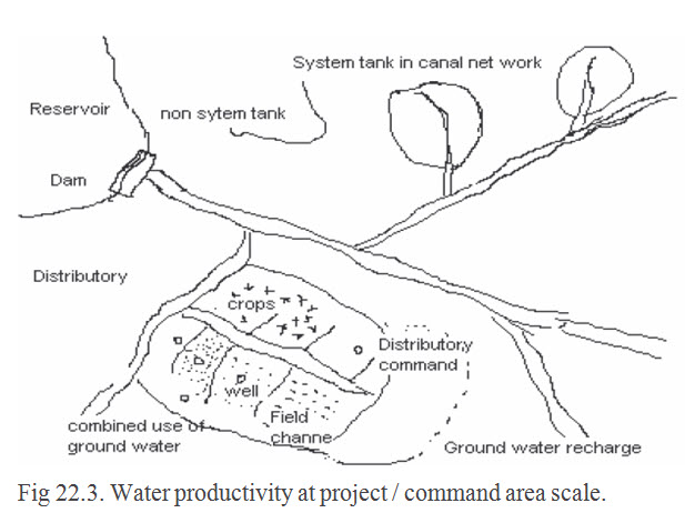
22.4. Project/Command area scale

In  Tamil  Nadu,  three  distinct  kinds  of  command  areas  are  in  vogue  viz.,  Canal  (or Reservoir)  command, Tank (system and non-system) command and Well (Groundwater) command. While the canal and tank commands mostly fall intact under a project operation, well commands occur in a scattered fashion.  When water is distributed in an irrigation system at a major scale like this, the important processes include allocation, distribution, conflict resolution and drainage. Allocation and distribution of irrigation water are primarily for irrigation farmers besides meeting the non-agricultural demands like domestic, industrial, livestock and fisheries use.

For canal command areas, irrigation scheduling cannot be done on a micro-scale calculating the depth of irrigation required, frequency of irrigation and the duration of irrigation owing to a larger areal extent with different crops and a different system of irrigation supply throughout the season on a rotational basis. Here, irrigation scheduling refers to the quantum of water to be stored or diverted for meeting the overall command area crop and allied demands. The water productivity concept shall be redefined by way of incorporating the overall irrigation efficiency and the duty of water at storage, flow and field level. The base period (B) over which irrigation flow is continuous through the canal network with suitable time rotations at outlets for distribution, also decide upon the productivity.

22.4.1. Canal command / Project Water Productivity (WP(c))

The overall productivity of this scale of reference depends ultimately on the total quantum of water released from storage over the base period, the area covered and the project yield. The storage duty (S) includes the losses during conveyance, distribution and application over and above the field duty (∆) in a canal network project.

Field duty (∆) is expressed as the seasonal water requirement for crop and related activities, in cm, at the tail most end area of the canal network.

∆= CU/η    -------(11)

where, η represents the farm/field efficiency  

Then, the  storage duty (S) = ∆/η_c  

Where, η_c  represents the overall conveyance efficiency of the canal network/ project

The flow duty (D) in ha/cumec is devised in accordance with S and ∆ to cover the given command area (A) over the base period (B) of the project water supply, as, 

D = (864B) / ∆  and S = A. ∆ / η_c          ----------(12)

As the command area/project scale is expanding the apparent losses like run-off and / or deep percolation would be considered for recycling or conjunctive use with canal flows. Then, the water productivity will be based on the total volume of water diverted from the irrigation source or simply the storage duty (S).

WP (c) = Y / S      ----------------------(13)

Where,

Y = project yield, in tonnes and

S = Storage duty, in ha.cm

If S is expressed in cm as S’ then, S’ = S/A

So that        WP(c)         = Y / S’       ----------   (14)

23.4.2. Tank Command Water Productivity WP (t):

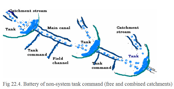
Nearly 39,000 tanks exist in Tamil Nadu State as natural surface water harvesting structures since the olden king regimes for the purpose of irrigation and other water usage. Earlier the tank system had clearly defined channel network originating from the storage outlet point and in due course of time these channels have disappeared owing to encroachments and other formidable reasons.  The tanks commonly come under a non-system (isolated or interconnected battery) with independent or combined catchments or a system tank arcade hooked along rivers or streams or canals, in which water at select points is diverted into the tank. Streams emanating from their own catchment basins during rains feed the non-system tanks and the water thus stored is utilized for irrigation and other purposes during the non- rainy season. In case of a battery of interconnected non-system tanks, water spilling from previous tank is diverted to the subsequent tank. System tanks are fed by flow diversion from natural river streams or from a project canal network as and when surplus flows occur. The gross volume of water depleted from the tank storage (Sd) or the equivalent depth (Sd’) in  cm,  over  the  crop  growth  season  forms  the  base  (denominator)  for   productivity calculations.

WP (t) = Y/Sd      -------------------------(15)

where,

Y = the overall tank command yield in tonnes

Sd = depleted volume of water from tank storage, ha.cm or Million cubic metres

Sd’ = equivalent depth in cm of water depleted from tank storage

 

23.4.3. Well Command Water Productivity WP (w)

Unlike the canal or tank commands, well commands are isolated and scattered and may also occur within a canal command or tank command. Absolute water productivity from an area fed by wells alone can be worked out if that area is away from a canal or tank command. But if the wells function within a canal or tank command, the conjunctive water productivity will be assessed on the premise that losses from canal or tank flows, contribute to groundwater recharge over a certain lag period i.e. loss is transformed into a gain. Recycling this gain of water  as  a  conjunctive use  of  groundwater  with  surface  waters  will  help  increase  the irrigation  area  thereby  increasing  the  absolute  productivity  of  the  region.  Water table fluctuations are periodically assessed to determine if the area comes under a dark zone or gray zone or a white zone for having exploited the groundwater potential and leading to a critical stage of minimum or controlled pumping with possibilities for introducing artificial recharge means and structures.  Water table fluctuations, pumping hours, discharge variations, power of pumping unit, mode of conveyance and application, type of crop and method of irrigation would contribute for the fluctuations in productivity. The productivity can be improved if lined channels or pipelines are used for conveyance and micro-irrigation systems are used for application.

WP (w) = Y/Wd   ----------------- (16)

Where,

Wd = volume or equivalent depth in cm of water depleted from well storage by pumping = (Pump discharge * total duration of pumping over the crop growth season) / Area of cultivation

All the above scales of reference shall be suitably formatted for input data, processing models and output units of productivity. The overall physical or economic productivity of a region shall then be worked out integrating the above scales.

Format 3. Water productivity at Project/Command area scale:

Project:       Tank/canal/Well

Command area (A)        :         ha

Crops and distribution area:   ha

Field duty (  ):      cm

Storage duty (S):  Mm3 ha.cm

Flow duty (D):     ha/cumec

Seasonal ET from entire command:  cm

(Use Penman- Monteith method)

Consumptive duty (C):                       Mm3 ha.cm

Storage – consumptive gap (S-C):      ha.cm

Over all project efficiency = ηo  = ηfc. ηdt. ηbc. ηmc.(1-ηgw)  ----(17)

ηfc     = Field channel efficiency

ηdt    = Distributory efficiency

ηbc    = Branch canal efficiency

ηmc   = Main channel efficiency

ηgw      = Ground water recharge efficiency (percolation loss from field)

S       = C/ηo    or                    ηo    = C/S

Project yield (physical crop wise) Yc  :         tonnes

Project economic yield: Yc’s equivalent income or monetary benefit (Ic)

WP (p) = Yc / S                or Ic / S                        --------------- (18)

22.5. Implications for integrated system water productivity

The physical water productivity (WPP) tends to decrease at a drastic rate towards the scale expansion to farm/field level from the ideal plant/crop level with the potential productivity. The reason attributes is runoff and deep percolation losses, resulting in reduced  efficiency  levels  and  an  increased  water  demand  at  the  field  inlet for diversion from the irrigation source.

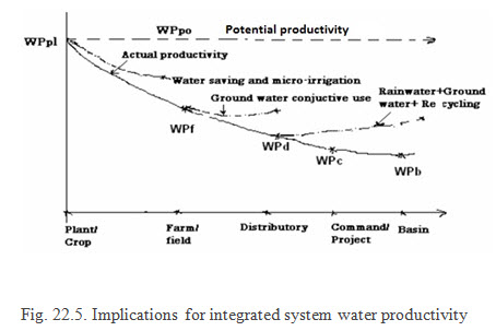From farm/field scale the rate of reduction in productivity decreases towards a distributory scale and thereupon it may attain constancy due to the effects of ground water conjunctive use and recycling from water harvesting structure for supplemental irrigation. Productivity can be improved upon by these effects.