System Engineering 3(3+0)

LESSON 2. Growth models

Use of growth models

Models are useful in drawing inferences.  When a scientist looks at a growth model, he will be able to draw the following inferences.

1. The exact relationship between time & growth.

2. The quantity growth at a specified point of time.

3. The rate of growth at each point of time.

4. In the case of perennial crops the asymptotic behaviour can be obtained.

5. The turning point in the growth can be estimated by so many methods.  A model can be estimated by so many methods.  But the best way of estimating a model is by the method of least squares.

1. Linear model

The general form of a linear model is y=a+bx.  Here both the variables x and y are of degree 1.  In a linear growth model, the dependent variable is always the total dry weight which is noted by w and the independent variable is the time denoted by t. Hence the linear growth model is given by w = a+bt.

2. To fit a linear model of the form  y=a+bx to the given data.

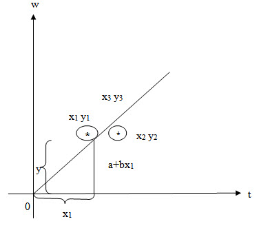
Here a and b are the parameters (or) constants of the model.  Let (x₁ , y₁) (x₂ , y₂)…………. (x_n , y_n) be n pairs of observations.  By plotting these points on an ordinary graph sheet, we get a collection of dots which is called a scatter diagram. 

In a linear model, these points lie close to a straight line. Suppose y = a+bx is a linear model to be fitted to the given data, the expected values of y corresponding to x₁, x₂…x_n are given by (a+bx₁) , (a+bx₂),………………… (a+bx_n).  The corresponding obserbed values of y are y₁ y₂……y_n. The difference between the observed value and the expected value is called a residual.  The Principles of least squares states that the constants occurring in the curve of best fit should be chosen such that the sum of  the squares of the residuals must be a minimum.  Using this for a linear model we get the following 2 simultaneous equations in a and b, given by

         ∑y = na+b∑x   --------------------------- (1)

         ∑xy = a∑x+b∑x² -------------------------(2)                    

         where n is the no. of observations.  Equations 1 and 2 are called normal equations. Given the values of x and y, we can find ∑x, ∑y, ∑xy, ∑x^2.    Substituting in equations (1) and (2) we get two simultaneous equations in the constants  a and b solving which we get the values of a and b

x	y	x2	xy
∑x	∑y	∑x2	∑xy

Note :If the linear equation is w=a+bt then the corresponding normal equations become

                        ∑w       =  na + b∑t      ------- (1)

                        ∑tw      = a∑t + b∑t²     --------(2)    

       

There are two types of growth models (linear)

(i) w = a+bt (with constant term)

(ii) w = bt (without constant term)

The graphs of the above models are given below :

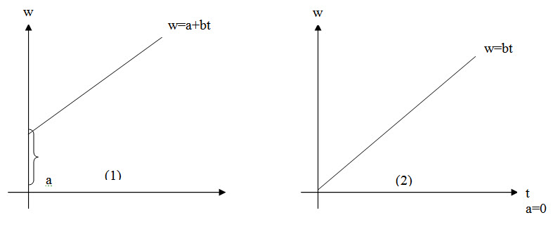
‘a’ stands for the constant term which is the intercept made by the line on the w axis. When t=0, w=a ie ‘a’ gives the initial DMP ie. Seed weight) ; ‘b’ stands for the slope of the line which gives the growth rate.

Exponential model

This model is of the form w=ae^bt where a and b are constants to be determined

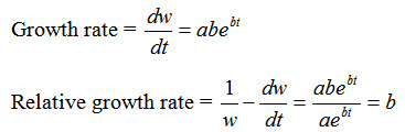
Here RGR = b which is also known as intensive growth rate or Malthusian parameter.

Note

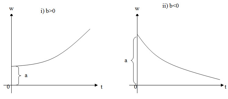
Population increases in geometric progression, whereas the food production increases in arithmetic progression.  In an exponential model the value of ‘a’ is always positive whereas ‘b’ can be positive or negative.  The graph of an exponential model is given below.

 

 

To find the parameters ‘a’ and ‘b’ in the above model first we convert it into a linear form by suitable transformation.

Now       w =  ae^bt    ----------------------(1)

Taking logritham on both the sides we get

            log_ew   =          log_e(ae^bt)

            log_ew   =          log_ea + log_ee^bt

            logw    =          log_ea + bt log_ee

            log w   =          log_ea + bt

            Y = A + bt      -------------------------(2)

Where Y = log w

            A = log_ea

Here equation(2) is linear in the variables Y and t and hence we can find the constants ‘A’ and ‘b’ using the normal equations.

            ∑Y = nA + b∑t

            ∑tY = A∑t + b∑t²

After finding  A  by taking antilogrithams we can find the value of a      

Note

The above model is also known as a semilog model.When the values of t and w are plotted on a semilog graph sheet we will get a straight line.  On the other hand if we plot the points t and w on an ordinary graph sheet we will get an  exponential curve.

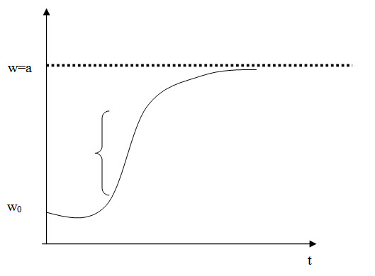
Logistic model : (or) Logistic curve

         The equation of this model is given by  \[w={a \over {1 + c{e^{ - kt}}}}\] -------------------- (1)

         Where a, c and k are constants.  The above model can be reduced to a linear form as follows :

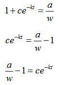
Taking logritham to the base e,

           

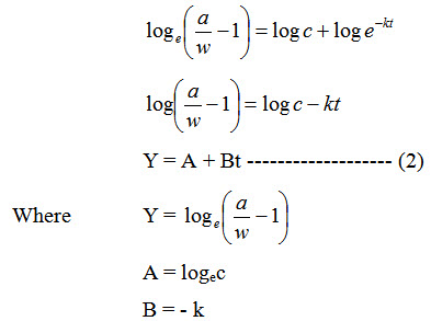
Now the equation (1) is reduced to the linear form given by equation (2) using this we can determine the constants A and B from which we can get the value of the constants c and k.

Note : I

Here’ a ‘ is called the carrying capacity. Either the value of ‘a’ is given or we assume the value of ‘a’ suitably.  The other two constants ‘c’ and ‘k’ can be obtained by solving the linear model 2.  The normal equations of the model 2 are :

                        ∑Y = nA + B∑t

                        ∑tY – A∑t + B∑t²

Solving these two equations we get the values of the constant A and B.