System Engineering 3(3+0)

Lesson 3 CLASSIFICATION OF QUEUING MODELS AND THEIR SOLUTIONS

Where

a = arrivals distribution

b = service time (or departures) distribution

c = number of service channels (servers)

d = max. number of customers allowed in the system (in queue plus in service)

e = queue (or service) discipline.

 

Certain descriptive notations are used for the arrival and service time distribution (i.e. to replace notation a and b) as following:

M = exponential (or markovian) inter-arrival times or service-time distribution (or    equivalently poisson or markovian arrivel or departure distribution)

D = constant or deterministic inter-arrival-time or service-time.

G = service time (departures) distribution of general type, i.e. no assumption is made about the type of distribution.

GI = Inter-arrival time (arrivals) having a general probability distribution such as as normal, uniform or any empirical distribution.

E_k = Erlang-k distribution of inter-arrival or service time distribution with parameter k (i.e. if k= 1, Erlang is equivalent to exponential and if k = , Erlang is equivalent to deterministic).

 

For example, a queuing system in which the number of arrivals is described by a Poisson probability distribution, the service time is described by an exponential distribution, and there is a single server, would be designed by M/M/I.

The Kendall notation now will be used to define the class to which a queuing model belongs. The usefulness of a model for a particular situation is limited by its assumptions.

 

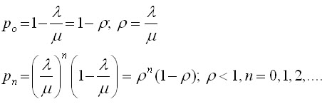
Model 1 :{( M/M1): (/FCFS)} single server, unlimited queue model

 

The derivation of this model is based on certain assumptions about the queuing system:

1. Exponential distribution of inter-arrival times or poisson distribution of arrival rate.
2. Single waiting line with no restriction on length of queue (i.e. infinite capacity) and no banking or reneging.
3. Queue discipline is ‘first-come, first-serve
4. Single serve with exponential distribution of service time

Performance characteristics

                  

       P_w   = probability of server being busy (i.e. customer has to wait) =  1-Ρ_{o= λ / µ}

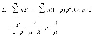
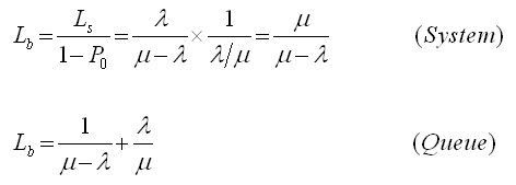
1.Expected (or average) number of customer in the system (customers in the line plus the customer being served)

 

 

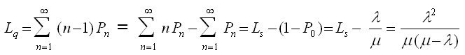
2.Expected (or average) queue length or expected number of customers waiting in the queue

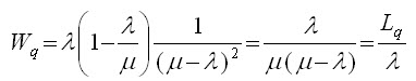
3.Expected (or average) waiting time of a customer in the queue

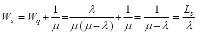
4.Expected (or average) waiting time of a customer in the system (waiting and service)

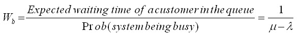
5.Expected (or average) waiting time in the queue for busy system

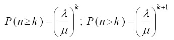
6.Probability of k or more customers in the system

7.The variance (fluctuation) of queue length

 Var (n) =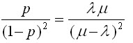 

8.Expected non-empty queue length

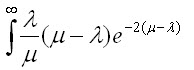
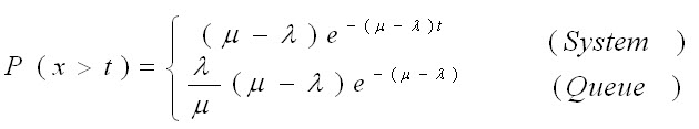
9.Probability that waiting time is more than

 ---------------------------------------------------------------

SOLVED EXAMPLES

 

Example1   A television repairman finds that the time spent on his jobs has an exponential distribution with mean of 30 minutes. If he repairs sets in the order in which they came in, and if the arrival of sets follows a Poisson distribution approximately with an average rate of 10 per 8-hour day, what is the repairman’s expected idle time each day? How many jobs are ahead of the average set just brought in?

 

Solution     From the data of the problem, we have

                   λ = 10/8 = 5/4 sets per hour;  and  µ= (1/30) 60 = 2 sets per hour

(a)  Expected idle time of repairman each day = Number of hours for which the repairman remains busy in an 8-hour day (traffic intensity) is given by

(8) (λ /µ ) = (8) (5/8) = 5 hours

Hence, the idle time for a repairman in an 8-hour day will be: (8 – 5) = 3 hours.

 

(b) Expected (or average) number of TV sets in the system

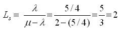  (approx.) TV sets

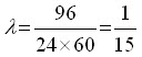
Example2   On an average 96 patients per 24-hour day require the service of an emergency clinic. Also on an average, a patient requires 10 minutes of active attention. Assume that the facility can handle only one emergency at a time. Suppose that it costs the clinic Rs 100 per patient treated to obtain an average servicing time of 10 minutes, and that each minutes of decrease in this average time would cost Rs. 10 per patient treated. How much would have to be budgeted by the clinic to decrease the average size of the queue from one and one-third patients to half patient.

 

Solution     From the data of the problem, we have

                  

                     and    patients per minute; 

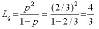
1.Average number of patients in the queue

2.Fraction of the time for which there no patients,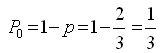 

3.When the average queue size is decreased from 4/3 patient, the new service rate is determined as:

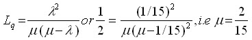  patients per minute.

Average rate of treatment required is: = 7.5 minutes, i.e.  a decrease in the average rate of treatment is 2.5(= 10 – 7.5) minutes.

 

Budget per patient = Rs (100 + 2.5 x 10) = Rs 125 per patient.

 

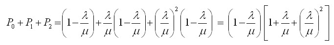
Example 3  Customers arrive at a one-window drive according to a Poisson distribution with mean of 10 minutes and service time per customer is exponential with mean of 6 minutes. The space in front of the window can accommodate only three vehicles including the serviced one. Other vehicles have to wait outside this space. Calculate:

 

(a)  Probability that an arriving customer can drive directly to the space in front of the window.

(b) Probability that an arriving customer will have to wait outside the directed space.

(c)  How long an arriving customer is expected to wait before getting the service?

 

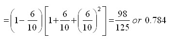
Solution     From the data of the Problem, we have λ=6 customers per hour; µ= 10 customers per hour

 

(a)  Probability that an arriving customer can drive directly to the space in front of the window:

 

(b) Probability that an arriving customer will have to wait outside the directed space:

 

 

(c)  Expected waiting time of a customer before getting the service is:

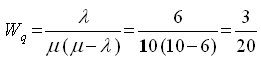 hr. or 9 minutes.