Site pages
Current course
Participants
General
MODULE 1. BASIC CONCEPTS
MODULE 2. SYSTEM OF FORCES
MODULE 3.
MODULE 4. FRICTION AND FRICTIONAL FORCES
MODULE 5.
MODULE 6.
MODULE 7.
MODULE 8.
LESSON 21.
21.1 Shear Force and Bending Moment diagrams for Cantilever subjected to different types of loading
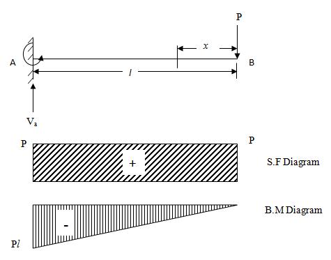
(i) Cantilever subjected to concentrated load ‘P’ at the free end
Fig.21.1 shows a cantilever AB fixed at A and free at B and carrying a load W at the free end B.
 \
\
Fig. 21.1
Consider a section X at a distance x from the free end
Shear Force (S.F) at X = Sx = + P
Bending Moment (B.M) at X = Mx = - Px
So, the S.F is constant at all the sections of the member between A and B.
But the B.M at any section is proportional to the section from the free end.
At x = 0 (at B), B.M = 0
At x = l (at A), B.M = -Pl
(ii) Cantilever with more than one concentrated load
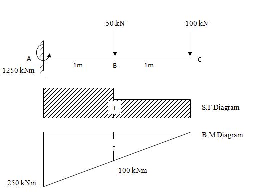
Fig. 21.2
Suppose a cantilever AC is 2 m long and is subjected to two concentrated loads.
Consider the section between B and C, distance x from C.
S.F = Sx= 100 kN
B.M = Mx = - 100x
At x = 0, Mx = 0
At x = 1, Mx = -100 kNm
Now consider section A and B, distance x from C.
S.F = Sx = 100 + 50 = + 150 kN
B.M = Mx = - 100x – 50(x-1)
= -150x + 50
At x = 1, Mx = -100 KNm
At x = 2, Mx = -250 KNm
(iii) Cantilever subjected to uniformly distributed load of p per unit run over the whole length
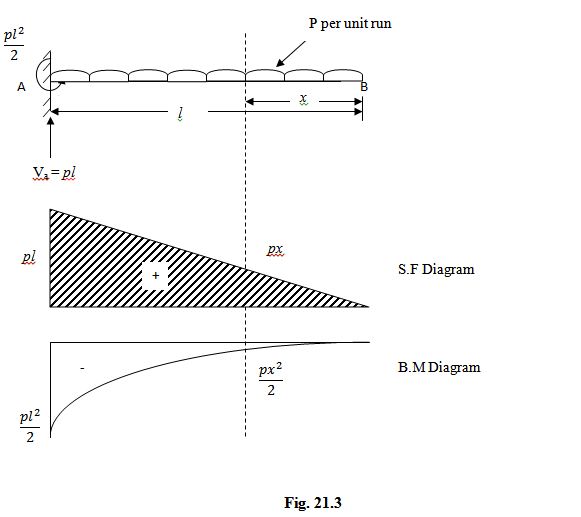
Fig.21.3 shows a cantilever AB fixed at A and free at B carrying a uniformly distributed load of w per unit run over the whole length.
Consider any section X distant x from the end B.
S.F at X = Sx = + px
B.M at X = Mx = - px . \[{x \over 2}\]
Therefore, Mx = - \[{{p{x^2}} \over 2}\]
- The variation of S.F is according to a linear law, while the variation of the bending moment is according to a parabolic law.
At x = 0, Sx = 0 and also Mx = 0
At x = l, Sx = + wl and Mx = - \[{{p{l^2}} \over 2}\]
(iv) Cantilever subjected to a uniformly distributed load of p per unit run for a distance a from the free end
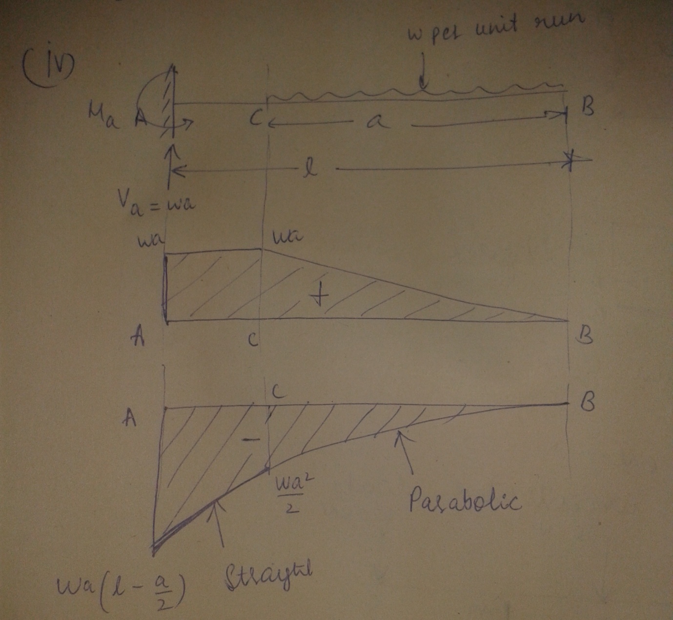
Fig.21.4
Fig.21.4 shows a cantilever AB fixed at A and free at B and carrying udl over a distance a.
Consider any section between C and B distant x from the free end B.
S.F, Sx = + px
B.M, Mx = - \[{{p{x^2}}\over 2}\]
The above relations are good for all the values of x between x = 0 and x = a
The variation of S.F will be linear and the variation of B.M for this section will be parabolic.
At x = 0, Sx = 0 and Mx = 0
At x = a, Sx = +pa and Mx = -pa \[\left({x-{a\over 2}}\right)\]
For section A and C, S.F is constant at +pa but the B.M varies according to linear law.
At x = a, Mx = -pa \[\left({a -{a\over 2}}\right)\] = \[{{w{a^2}}\over 2}\]
At x = l, Mx = - pa \[\left( {L - {a \over 2}} \right)\]
(v) Cantilever subjected to a uniformly distributed load w per unit run over the whole length and a concentrated load P at the free end.
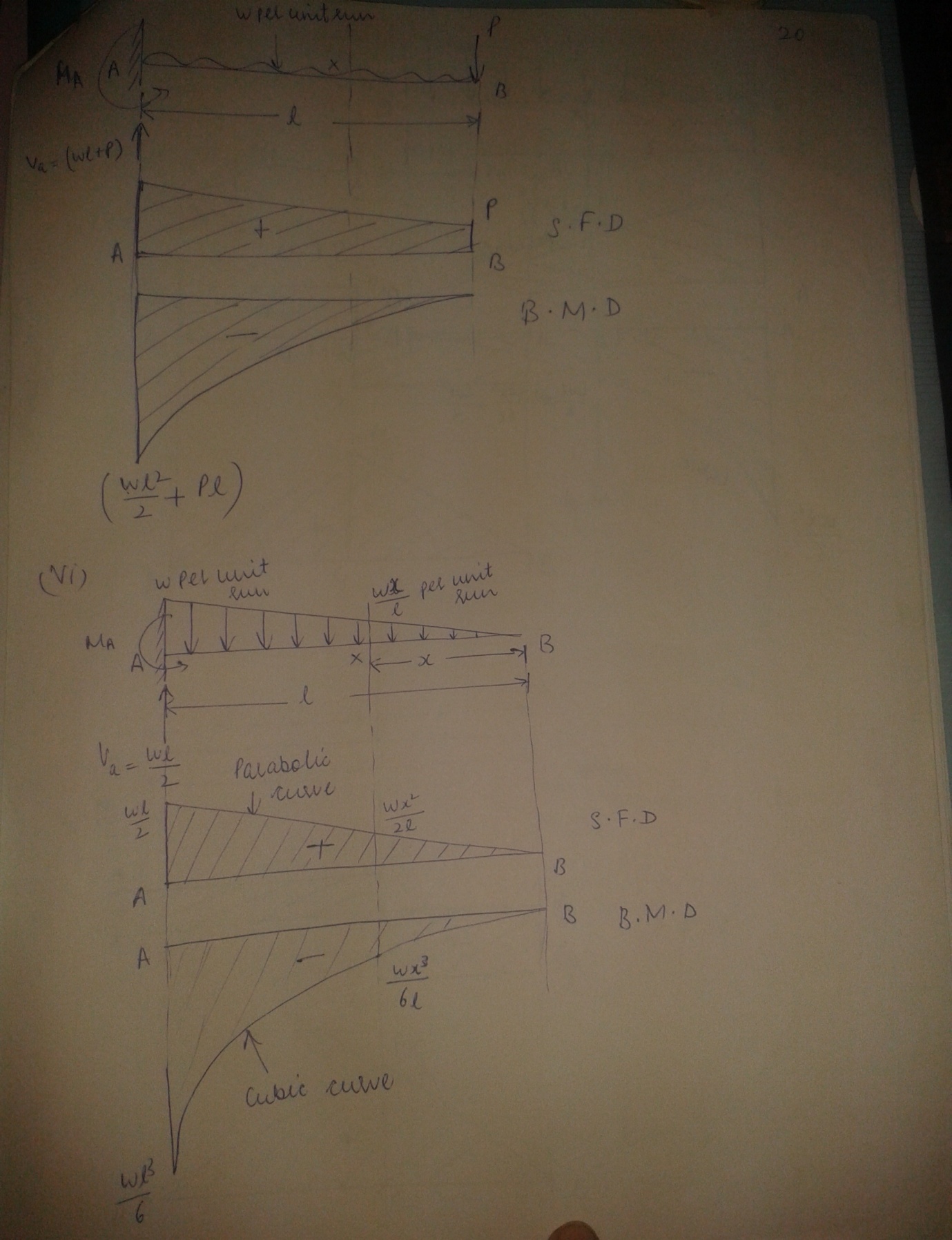
Fig. 21.5 and 21.6
Fig.21.5 shows a cantilever AB fixed at A and free at B and carrying the load system mentioned above. Consider any section X distant x from the end B. The S.F and the B.M at the section X, are respectively given by.
Sx = wx + P
And Mx = - \[\left( {{{w{x^2}} \over 2} + Px} \right)\]
At x = 0, Sx = + P and Mx = 0
At x = l, Sx = + (wl + P)
Mx = - \[\left( {{{w{x^2}} \over 2} + Pl} \right)\]
(vi) Cantilever subjected to a load whose intensity varies uniformly from zero at the free end to w per unit run at the fixed end
Fig.21.6 shows a cantilever AB of length l fixed at A and free at B carrying the load as mentioned above.
Let the intensity of loading at X, at a distance x from the free end B be wx per unit run.
Therefore wx = \[x \over l}w\] since the intensity of load increases uniformly from zero at the free end to w at the fixed end.
The total downward load on the free body, equal to the area of the triangular loading diagram (Fig.21.6), is
\[+{1\over 2}\left({{{{w_x}}\over l}}\right)\left( x \right)=+{{w{x^2}} \over {2l}}\]
Sx \[+{{w{x^2}} \over {2l}}\]
Mx = Moment of the load acting on XB about X
= area of the load diagram between X and B × distance of the centroid of this diagram from X
\[=-{{w{x^2}} \over {2l}}.{x \over 3}\]
Mx = \[-{{w{x^3}} \over {6l}}\]
At x = 0, Sx = 0 and Mx = 0
x = l, Sx = \[+ {{wl} \over 2}\] and Mx = \[- {{w{l^2}} \over 6}\]
The S.F varies following a parabolic law while the B.M follows cubic law.
(vii) Cantilever subjected to a load whose intensity varies unifrormly from zero at the fixed end to w per unit run at the free end
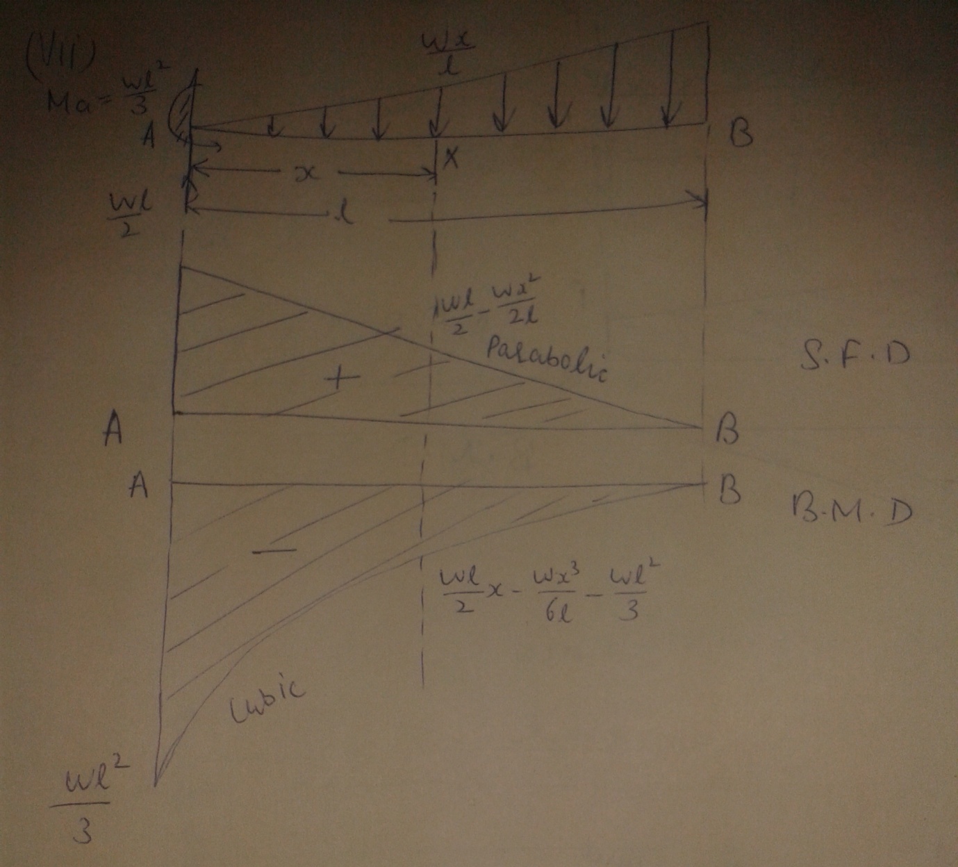
Fig. 21.7
Fig.21.7 shows a cantilever AB of length l and fixed at A and free at B and carrying the loading as mentioned above
Let Ma be the reacting moment of fixing moment A.
Therefore Ma = moment of the total load amount A
= \[{{wl}\over 2}.{{2l} \over 3}={{w{l^2}} \over 3}\]
Va = vertical reaction at A
= Total load on the cantilever
Va = \[{{wl}\over 2}\]
Consider any section X distant x from the fixed end A
S.F at X = algebraic sum of forces on AX
Sx = \[{{wl}\over 2} - {x \over 2}.{{wx} \over l}\]
Sx = \[{{wl}\over 2} - {{w{x^2}} \over {2l}}\]
B.M at X = algebraic sum of forces and reactions on AX above X
Mx = \[{{wl} \over 2}x - {{w{x^2}} \over {2l}}.{x \over 3} - {M_a}\]
= \[{{wl} \over 2}x - {{w{x^3}} \over {6l}} - {{w{l^3}} \over 3}\]
At x = 0 i.e at A, Sx= + \[{{wl} \over 2}\] and Mx = - \[{{w{l^2}} \over 3}\]
At x = l i.e at B, Sx = \[{{wl} \over 2}\] - \[{{w{l^2}} \over 2l}\] = 0 and Mx= \[{{wl} \over 2}l - {{w{l^3}} \over {6l}} - {{w{l^3}} \over 3}=0\]
Example: Fig.21.8 shows a cantilever subjected to a system of loads. Draw S.F and B.M diagrams.
Solution: At any section between D and E, distance x from E
S.F = Sx = +500 N
B.M = Mx = -500x
At x = 0, Mx = 0
x = 0.5m, Mx = -250 Nm
At any section between C and D, distance x from E
S.F = Sx = +500 + 500 = + 1000 N
B.M = Mx = -500x – 500(x - 0.5)
= -1000x + 250
At x = 0.5, Mx = -250 Nm
At x = 1m , Mx = -750 Nm
At any section between B and C, distance x from E
S.F = Sx = +500 + 500 + 400 = + 1400 N
B.M = Mx = -500x – 500(x - 0.5) – 400(x – 1)
= -1400x + 650
At x = 1m, Mx = -750 Nm
At x = 1.5m , Mx = -1450 Nm
At any section between A and B, distance x from E
S.F = Sx = +500 + 500 + 400 + 400 = + 1800 N
B.M = Mx = -500x – 500(x - 0.5) – 400(x – 1) – 400 (x – 1.5)
= -1800x + 1250
At x = 1.5m, Mx = -1450 Nm
At x = 2m , Mx = -2350 Nm
Last modified: Tuesday, 10 September 2013, 10:48 AM