Engineering Chemistry 3(2+1)

Lesson 31. Fibre and Rubber materials

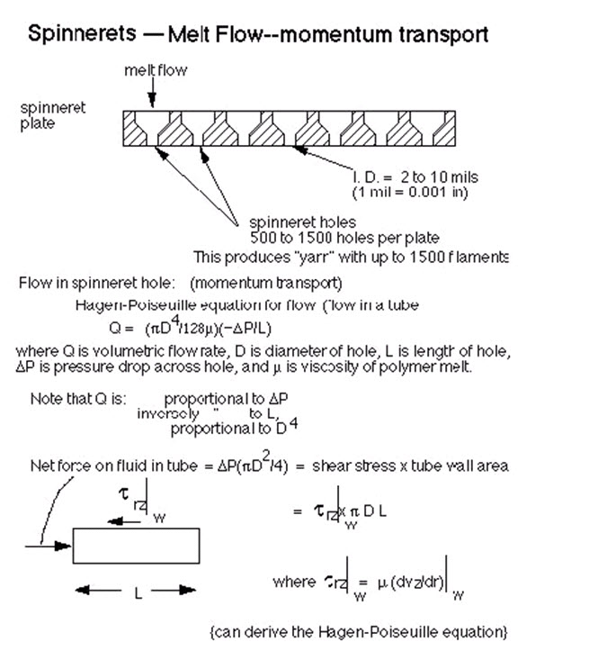
As mentioned previously, fibers are formed by the extrusion of the polymer melt or spin dope through tiny holes in a spinneret plate.  Such a plate may contain 1,000 holes or more. Textile fibers are relatively fine, so the diameter of the hole may be only a few mils, where one mil is 0.001 inches (25.4 μm). The thickness of the filament is generally not given in linear dimensions, but rather in terms of mass per length. For some reason the fiber industry has adopted the terms denier and denier per filament, dpf, to express the filament size. One dpf corresponds to a mass of 1 g in a length of 9000 meters ! If the density of the polymer is 1 g/cm³, this would correspond to a diameter of 1.2 x 10^-3 cm, or about half a mile. Typically, textile fibers are in the range of 3 to 15 dpf. Recall that one gm is roughly 1/30  of an ounce. In melt spinning, the filaments are normally drawn down, or stretched, just downstream of the spinneret holes. The stretch is of the order of 2 to 3x, so the spinneret hole may be 50 to 75% larger than the filament diameter when it is first cooled.

Additional post formation stretching may also be used, however, so that the final filament diameter may be one-half or less than the diameter of the spinneret hole. The spinneret hole is usually only slightly longer than its width, in part to minimize pressure drop at the plate. But the plate still has to be strong enough to withstand the upstream pressure. For this reason, the melt passes through a conical section before reaching the final spinneret hole, so that the plate can be relative thick (see slide). Pressure drop through this converging section is very difficult to calculate for these polymeric materials, because the extensional flow rheology is usually not well characterized. One can readily visualize the alignment of the polymer molecules in the converging section, where the polymer undergoes a severe stretching step. Ignoring this pressure loss, let us focus on the spinneret hole itself.

An important question here is whether one can use the Hagen-Poiseuille equation to compute the pressure drop in such a short tube. To help answer this question, we first compute the entrance length, which is approximately equal to the axial distance downstream from a tube entrance at which the momentum boundary layers merge at the center axis, where a fully parabolic profile is established. This distance, from Bird, Stewart, and Lightfoot, Transport Phenomena, p. 47, is Le/D = 0.035 Re (4-1).

where Le is the entrance length, D is the tube diameter and Re is the Reynolds number.

 

For a representative calculation, we consider nylon melt, with a viscosity of 200 Poises, being spun from a hole 10 mils in diameter at a final spinning speed of 2,000 ypm and a stretch of 5x between the spinneret and the final take-up. This means that the bulk velocity, ub, in the spinneret hole is 400 ypm. The Reynolds number, for a specific gravity of about one, is:

Re = ub D/n = 0.077

so the entrance length is less than 3 thousandths of the diameter of the hole. Therefore, we can safely use the Hagen-Poiseuille equation to calculate the pressure drop.

 For the nylon example we just explored, the pressure drop is predicted, for a length of 3.0 mils, to be 2200 psi. This pressure drop might be a bit excessive in practice, but the method of calculation remains illustrative. One part of the calculation which was not taken into account is the power-law behaviour of most polymer melts and polymer solutions. Such behaviour usually is revealed by a shear-thinning response, in which the apparent viscosity decreases as shear rates increase. This would lead to significantly lower pressure drops for the spinneret plate.

As the polymer exits the spinneret hole, it tends to swell and this swell is especially noticeable at low filament tensions. Apparently, the polymer molecules must coil under the shearing action within the hole and, as it exits, the polymer molecules are free to uncoil, as seen by an expansion of the polymer stream jetting out of the hole. This phenomenon is referred to as "die swell," and can even amount to a doubling or more of stream diameter. Even Newtonian fluids can be shown to exhibit a swelling at the exits of tubes, even at very low Re; the predicted extent of swell is about 14% for Newtonian fluids. Since, in fiber spinning, the filaments are under tension, the extent of die swell is considerably reduced. Furthermore, the extent of swell appears to have no influence of final filament properties. In order for the filaments to undergo stretching, some power must go into the stretching motion immediately downstream of the spinneret plate, but the amount of this power is negligible.

 MELT SPINNING

In the spinning of molten polymers, such as nylon, polyester, and polypropylene, melt spinning begins with a cooling of the molten filament after it leaves the spinneret. At the same time, the filament is pulled downwards towards the take-up section and this resulting tension in the molten filament provides a stretching action in the molten filament itself. In most melt spinning operations the degree of stretch is of the order of 3x, which means that the velocity of the initially cooled, or solid, fiber is about three times the average velocity of the melt coming out of the spinneret. For some filaments, this initial stretch is very important in helping to establish properties in the polymer which depend on whether one deals with the properties in the fiber axis direction or in the fiber radius direction. This directional dependence of properties is called anisotropy and the usual example is that of a slab of wood, in which strength and fracture properties along the grain are quite different from properties across the grain. (With many fibers, however, these properties are controlled downstream, where the fibers are reheated, stretched further, and cooled again).

In any case, the polymer melt, once it comes out of the spinneret hole, starts to cool down and also starts to stretch out. Because the "apparent viscosity" of the melt increases rapidly as the melt cools, most of the stretching takes place in a region relatively close to the spinneret hole whereas "most" of the cooling takes place well away from this hole. But these terms and descriptions are not exact and are not easily quantified. The real advantage in using these descriptions is that it permits us to make a simplifying assumption as we analyze the melt spinning process. The assumption is: We can separate the stretching and cooling operations into two separate distinct regions, with the first occurring relative close to the spinneret (say, within 10% of the distance to the first take-up, or speed-control roll), and the second over the remaining distance to the first take-up roll. If need be, we could return later to this assumption to determine its degree of accuracy, but let us accept it for the moment.

The stretching region, within which the relatively long polymer molecules become aligned along the filament axis, might be characterized by very complex rheology. Within the field of polymer processing, rheology deals with the relationship between stress and the history of strain; for Newtonian fluids, you can recall that the fluid stress is proportional to the rate of strain (the shear rate). We are not really too concerned about the polymer melt rheology here, however, since it will not likely be important in determining the power required for the first drive or take-up roll. Frictional and interfacial stresses are likely to be far more important. Therefore, in terms of design considerations, we can probably ignore that part of the melt-spinning process in which the initial, post-spinneret stretching of the polymer melt occurs and focus instead on the cooling step of the melt spinning operation.

Perhaps the most important design consideration in the melt spinning process is the cooling of the filaments. In order to simplify our analysis, we restrict our focus to the point where the filaments have reached a uniform diameter (recall that we previously asserted that this is a relatively short distance) and that they are at some initial temperature which will be somewhat cooler (by about 20 C°) than the melt temperature at the spinneret exit. At this point, the temperature within the filament will depend on radial position, with the maximum occurring at the center, on the filament axis. We shall invoke an pproximation of a flat temperature profile, in which the temperature does not vary with r, in order to utilize existing mathematical solutions.

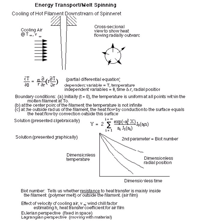
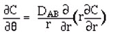
An important part of learning engineering is to learn how to take "appropriate shortcuts" which save time with little sacrifice in accuracy. This is one example. The melt spinning process is steady: viewing the spinning threadlines at a fixed position (the so called Eulerian perspective) shows that nothing appears to change with time. If one situates oneself on the moving threadline (figuratively, of course) there does certainly appear to be a time dependence to the temperature of the filament. This viewpoint of moving with the material is called the Lagrangian perspective. Whereas the Eulerian perspective requires you to measure the threadline temperature as a function of r, radial position within the filament, and z, axial position along the filament, in order to follow the cooling, the Lagrangian perspective allows you to follow the cooling as a function of r and t, where t is time. Zero time should be some convenient reference-here it would correspond to locating yourself on the filament at the end of the stretching region and at the "beginning" of the cooling region. This is equivalent to the cooling of an infinite rod which is fixed in space. The governing differential equation, which can be derived easily using shell balance techniques is:

where q is time and a is the thermal diffusivity of the polymer. The student will readily recognize this as a partial differential equation, since the temperature T depends on both r and q. In order to solve the equation quantitatively, one must specify initial and boundary conditions. The boundary is naturally R the outside radius of the filament. So the initial condition ( q = 0)is simply:

T (r,q) = To for r< R ,where To is a constant.

We need two boundary conditions, corresponding to r = 0 and r = R. At r = 0,

T remains finite;

At r = R, the heat arriving at the surface by conduction from within must match the heat

leaving by convection:

at r = R and all q > 0. k is the thermal conductivity of the filament (we shall assume that this conductivity does not change as the polymer solidifies. h is the heat transfer coefficient governing the heat transfer from the surface to the surrounding air. An example of such a correlation for heat transfer from a cylinder in crossflow is given by Churchill and Bernstein

where NuD is the Nusselt number, hD/k, (k is the thermal conductivity of the fluid in crossflow and D is the cylinder diameter) and ReD is the Reynolds number based on the fluid in crossflow. Pr is the Prandtl number, n/a,and is also based on the crossflow fluid. The student will recall that an important advantage of presenting correlations in terms of dimensionless variables like Nu (dimensionless heat transfer coefficient) and Re (inertial stresses divided by viscous stresses) is that the resulting expression is often simpler, revealing more clearly the relationships among such variables.

We shall also assume that the heat of fusion is negligible, primarily because we want to simplify the calculation. This assumption, especially for crystalline polymers, could be very poor, however, and could lead an underestimate of the cooling time by a factor of two.

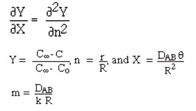
As engineers, or even as normal, sane people, we would not want to solve the differential equation for every single set of geometries, thermal diffusivities and initial and boundary conditions. We can avoid this needless energy expenditure if we express the differential equation in dimensionless form:

Y is called the unaccomplished temperature change, since it starts at unity at time zero and declines from there. n is the normalized radial position, and X is dimensionless time, sometimes called the Fourier number. One final dimensionless group, m, expresses the relative resistance outside the filament to that in the filament:

Finally, the initial and boundary conditions become:

Y = 1 at X = 0 and 0 < n < 1;

at n = 0 and X > 0.

at n = 1 and X > 0.

The solution, Y(n, X) is then valid for any case of unsteady-state heat conduction within a cylindrical geometry with a uniform initial temperature and convective heat transfer from the surface to a surrounding fluid at a uniform temperature T . The solution is shown in graphical form on the slide and is available in almost all transport textbooks. The resulting charts are known variously as "Gurney-Lurie Charts" or "Heissler Charts," depending on which reference or form of charts you use. An analytical solution for a slightly less general case is given below. Note that, by use of dimensionless variables, we have successfully created a result which is applicable to a broad range of geometries and material properties. For the special case in which heat transfer resistance from the surface of the fluid to the surrounding fluid is negligible, one can set h, the heat transfer coefficient, to (this, of course, is equivalent to setting the temperature of that surface to that of the surrounding fluid for all q > 0) and the analytical solution is:

where J0 and J1 are Bessel functions of the first kind (zero and first order, respectively), and ai is the ith root of J0(ai) = 0. This solution is presented in the transport text Momentum, Heat, and Mass Transfer, by Bennett and Myers, 3rd ed., p. 286.

 

Key elements that you have learned in this section include:

Difference and relationship between Lagrangian and Eulerian perspective, Existence of unsteady-state heat conduction charts, Heat transfer resistance within objects relative to resistance outside these objects, Value of dedimensionalization as a means to obtain more general solutions to complex equations, A typical heat transfer correlation for heat transfer coefficient, h.

Spinning of synthetic fibers with a melt spinning process is conceptually simple, involving little more that the extrusion of molten polymer through fine holes and solidification of the resulting filaments by cooling.

 

DRY SPINNING

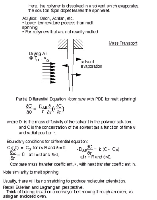
Unlike melt spinning, both dry and wet spinning use solvents in which the polymer dissolves. The resulting solution or suspension is a viscous "spin dope." This process necessarily introduces another species, which is subsequently removed, and therefore is more expensive than conventional melt spinning processes. It is used in cases where the polymer may degrade thermally if attempts to melt it are used or in cases where certain surface characteristics of the filaments are desired-melt spinning produces filaments with smooth surfaces and dry spinning produces filaments with rough surfaces. The rougher surface may be desirable for improved dyeing steps or for special yarn characteristics.

The term "dry spinning" is a bit misleading, since the polymer is certainly wet by a solvent. Presumably, the intent here was to distinguish the two methods of solvent removal for the two cases of dry and wet spinning. The solvent in dry spinning is a volatile organic species and this solvent starts to evaporate after the filament is formed, which is immediately downstream of the spinneret. Whereas melt spinning involved solidification by cooling, dry spinning produces solidification of the polymer by solvent removal.

Several commercial fibers, including acrylic fibers such as Orlon™, are made by a dry spinning process. You may recall that these acrylic fibers are popular as substitutes for wool fibers. In any case, the spinning step which defines, in large part, the spinning process is that of solvent removal from the filaments. In the case of Orlon, the polymer, polyacrylonitrile, is dissolved to a polymer concentration of 20 to 30 wt% in a dimethylformamide solvent. Warm gases (air - probably not, on account of the need for solvent recovery) are passed through the fiber bundle in the region just downstream of the spinneret.

This begins to look very much like the cooling crossflow in melt spinning. The solvent encounters both a diffusional resistance within the fiber and a convective resistance in moving from the surface of the filament to the crossflow gases.

Within the filament, the material property of greatest importance is DAB, the diffusivity of the solvent A through the filament here; we can characterize the diffusive flux of the solvent by:

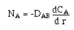
which is your familiar Fickian Diffusion equation. We use the ordinary derivative here because the process is steady and we have not yet begun to use the Lagrangian perspective we have.

 One point to emphasize here is the similarity of this equation to the Fourier heat conduction equation. If we then adopt the Lagrangian perspective, we have Comparison with the unsteady heat conduction equation reveals the equation to be identical with the exception that “a” is replaced by DAB and T by C. Both “a” and DAB have dimensions of length squared over time or units of cm²/s. The initial and boundary conditions are also practically identical to the heat transfer case, with the assumption of uniform concentration profile at time zero, and zero concentration gradient on the filament centerline and matching diffusive and convective flux at the filament surface:

C (r,0) = Co  for   r< R and q = 0,

at r = 0 and q>0

and

at r = R and q>0

Instead of heat transfer coefficient, h, we have mass transfer coefficient, k. Correlations for k, expressed in terms of a dimensionless mass transfer coefficient, Sh (for Sherwood number) as a function of ReD and Sc, are also available. Sc is the ratio of momentum diffusivity to mass diffusivity, n/DAB, (for the cross flow fluid) and is comparable to the Prandtl number, n/a. Note that n and DAB are the momentum diffusivity and mass diffusivity of the gas in crossflow, and not of the polymer solution. One correlation for “k” is:

Sh = 0.281 (ReD)-0.4 where Sh = (kD/DAB). This correlation is a bit unusual, in that normally the mass transfer coefficient is found to be proportional to the diffusivity raised to a power less than unity. The reader may want to check other correlations to check whether this form may or may not be reasonable.

Just as we dedimensionalized the heat transfer equations, we can do the same for solvent diffusion. The resulting equations then are exactly identical to those for unsteady heat conduction.

 

Of course, T is replaced by C, a by DAB, h by k. Therefore, the same solution (graphical or analytical) is obtained and the same charts can be used to obtain quantitative predictions of the fiber spinning process. One can readily calculate, therefore, the Fourier number, X, required for the solvent concentration at the filament centerline to become less that 1% of the original value (Y < 0.01). From this value for X, the actual time (in a Lagrangian sense, remember) can be calculated. Finally, by multiplying this time by the yarn speed, the length of the solvent recovery section is obtained directly. The analogy here might be that of using a conveyor belt in a tunnel oven to bake bread. We can calculate the length of the tunnel oven, once we know the time to bake the bread and the speed of the conveyor belt.

 Wet Spinning

Fibers produced by wet spinning include rayon and Kevlar. Rayon was originally developed as a synthetic substitute for silk and Kevlar was produced as a high-strength fiber for use in various aerospace and specialty-use applications. Furthermore, many commercial acrylic fibers are also produced by wet spinning.

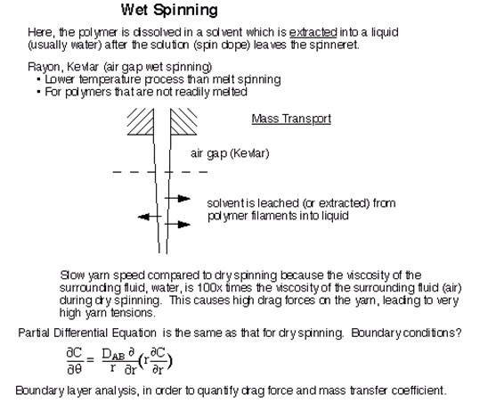
As with dry spinning, the polymer is dissolved or suspended in a solvent, to form a viscous "spin dope" and filaments are formed by extrusion through tiny holes in a spinneret plate. Kevlar, for example, will degrade thermally if attempts are made to melt it, and thus a solvent must be used. With wet spinning, the term more accurately depicts the process than with dry spinning, because the solvent is extracted or, perhaps more appropriately, leached, from the filaments by another liquid. In most cases, the second liquid is aqueous.

A major difference between wet spinning and either melt or dry spinning is that one is spinning into a fluid (liquid) with a much higher viscosity. Because this higher viscosity can translate into high shearing stresses on the surfaces of the filaments, the tension in the filaments can become quite high. For example, towing a buoy by a long line behind a boat can produce very high tensions in the line when compared with towing the same buoy by a short line. For long baths, the tension can become sufficiently high that the filaments might break, as their tensile strength is exceeded. To avoid this danger, much lower spinning speeds must be used. Whereas melt spinning may utilize spinning speeds of 2,000 yards per minute (80 mph), spinning speeds in wet spinning are usually less than 300 ypm.

Another difference with dry spinning is the capability of using many more spinneret holes in the case of wet spinning. The total number can approach 60,000 in a single spinneret plate, if the spinning is done directly into a coagulating or extracting liquid. Because the liquid is present, the filament forms a type of skin almost immediately and the potential for the filaments to touch and fuse is practically eliminated, compared with dry or melt spinning.

In the case of Kevlar the spin dope is relatively warm, about 100°C, and forms a viscous, liquid crystal. The solvent is sulfuric acid, at a concentration of about 80 wt% (20 wt% polymer). These liquid crystals are easily oriented by a stretching

motion. Therefore, during the spinning process, the filaments are first extruded through an air gap, where the filaments undergo strains of 2 to 3x, which produces a high degree of molecular orientation in the filaments. This air gap is of the order of one inch. It also allows the spinneret plate to be warm (100°C) while the extraction bath can be cool (ca 15°C). The hot filaments then strike the cooling bath where the filaments are "quenched" and much of the orientation is locked in by the rapid cooling action. Subsequent to the quench step, the solvent is extracted, which requires a relatively long bath contact time. But the initial quenching step is crucial, since it allows for the oriented molecules to be "frozen" into position. This orientation is particularly important to the high-strength properties of Kevlar-the filaments, on a weight basis, are stronger that steel, almost by a factor of two. If one attempts to use the same process to produce Kevlar filaments of large diameter, the core of the filaments can lose its orientation, because the quench time to reach the core will increase with the square of the filament radius. The filament skin, or the outer part of the filaments, however, will have the orientation locked in and a high degree of orientation will exist there. This produces a so-called "skin-core" effect, in which the average properties of the filaments, expressed as tensile strength per unit cross-sectional area, will decline on account of a decreased average orientation. Kevlar, with its focus on strength development via "air-gap" wet spinning, is somewhat unique within the process of wet spinning. As with melt- and dry- spinning, the controlling part of the process is associated with development of the filament structure, either by cooling of the filament or by removal of the solvent. The equations for diffusion in wet spinning are identical to those for dry spinning, with the exception that the fluid passing outside the filaments is a liquid and not a gas.

Also, the flow may not be across the filaments, but even, partially, along the filaments. Therefore, the correlations and nature of the flow surrounding the filaments will result in different values for the surface mass transfer coefficient. Whether this will change the relative resistance dramatically will depend on the particular fiber to be produced and its dimensions and properties. The same graphical solutions described earlier can be used, however, to design a wet-spinning process, it may be necessary to predict the transport of momentum, heat, and mass in the region adjacent to the filament just downstream of the spinneret. One can use a so-called "boundary-layer" analysis to do this.

Treatment of such an analysis is beyond the scope of the present discussion of fiber spinning, but a brief description of the analysis is appropriate. One form of boundary-layer analysis involves von Karman integral boundary-layer techniques. The boundary layer starts at zero thickness at the first point where the fiber contacts the extracting liquid, and growing gradually radially outwards from each filament as one proceeds downstream. The velocity profile inside the boundary layer is assumed and all of the velocity change between the filament and the surrounding fluid is contained within this "momentum" boundary layer. Similarly, thermal and diffusional boundary layers contain all the changes in temperature and concentration, respectively. Based upon approximations of these velocity profiles, frequently assumed to be turbulent, the variation in filament drag with position can be predicted, along with local heat and mass transfer coefficients. The student is referred to Transport Phenomena, by Bird, Stewart, and Lightfoot, for additional details of such integral boundary-layer techniques.