Engineering Properties of Biological Materials and Food Quality 3(2+1)

Lesson 11. Stress relaxation and Creep behaviour

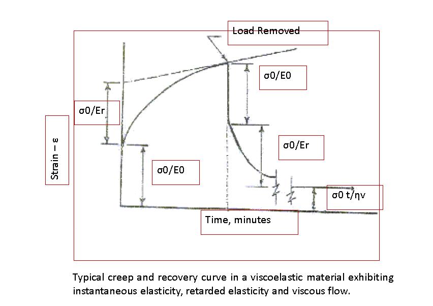
Creep: Deformation with time when the material is suddenly subjected to a dead load-constant stress.

Retardation time: The rate at which the retarded elastic deformation takes place in a material creeping under dead load. It is the time required for the Kelvin model, representing creep behavior, to deform to (1-(1/e)) or about 63 percent of its total deformation.

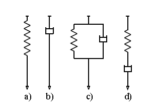
The mechanical models

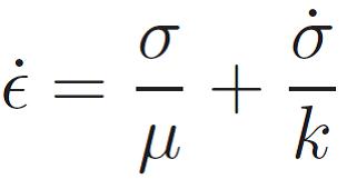
To get some feeling for linear viscoelastic behaviour, it is useful to consider the simpler behaviour of analog mechanical models. They are constructed from linear springs and dashpots, disposed singly and in branches of two (in series or in parallel). As analog of stress and strain, we use the total extending force and the total extension. We note that when two elements are combined in series [in parallel], their compliances [moduli] are additive. This can be stated as a combination rule: creep compliances add in series, while relaxation moduli add in parallel.

The Hooke model: The spring (Fig. a) is the elastic (or storage) element, as for it the force is proportional to the extension; it represents a perfect elastic body obeying the Hooke law (ideal solid). This model is thus referred to as the Hooke model. If we denote by m the pertinent elastic modulus we have Hooke model : σ(t) = mǫ(t),

In this case we have no creep and no relaxation so the creep compliance and the relaxation modulus are constant functions: J(t) ≡ Jg ≡ Je = 1/m;

G(t) ≡ Gg ≡ Ge = m

Newton Model: The dashpot (Fig. b) is the viscous (or dissipative) element, the force being proportional to rate of extension; it represents a perfectly viscous body obeying the Newton law (perfect liquid). This model is thus referred to as the Newton model. If we denote by b1 the pertinent viscosity coefficient, we have

Newton model : σ(t) = b1(dǫ/dt)

J(t) = t/b1 , G(t) = b1 δ(t)

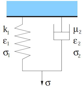
KELVIN-VOIGT MODEL

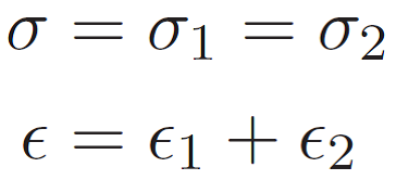
Kelvin-Voigt viscoelastic solid element consists of a Hookean elastic element (HE) and a Newtonianviscous element (NE) connected in parallel fig. c. In a Kelvin-Voigt model, the resulting stress is the sum of the components of stress carried by the elastic element (σ1) and the partial stress carries by the Newtonian viscous element (σ2 ). A branch constituted by a spring in parallel with a dashpot is known as the Kelvin–Voigt model.

\[\sigma={\sigma _1} + {\sigma _2}= k\varepsilon+\mu\dot\varepsilon\]

\[\varepsilon={\varepsilon _1} ={\varepsilon _2}\]

The retardation time is basically a measure of the degree of elastoviscosity of a material and hence governs the degree of rigidity (or fluidity) of a viscoelastic material. A very low retardation time indicates the material to be a highly elastic solid. In such a condition, the material behaves as a rigid body. On the other hand, when the retardation time is very high, the viscous property of the material overpowers the elastic property. Under such conditions, the material behaves as a fluid with instantaneous initial rigidity.

It is also understood that the presence of a viscous dashpot in parallel to an elastic element significantly reduces the magnitude of strain generated in the viscoelastic element. The Kelvin-Voigt model exhibits an exponential (reversible) strain creep but no stress relaxation; it is also referred to as the retardation element.

• Handles creep fairly well

• Handles Recovery fairly well

• Does not account for relaxation

MAXWELL MODEL

The spring and dashpot are connected in series (fig. d).

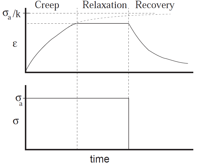
If the stress σ =σ_o does not vary with time i.e. the element is subjected to a constant stress, the element undergoes creep. The total strain at any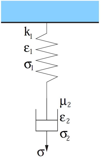

instant of time e is expressed as a summation of instantaneous elastic strain e₁and the creep strain (e₂) defined by the following expression

Stress and Strain are connected as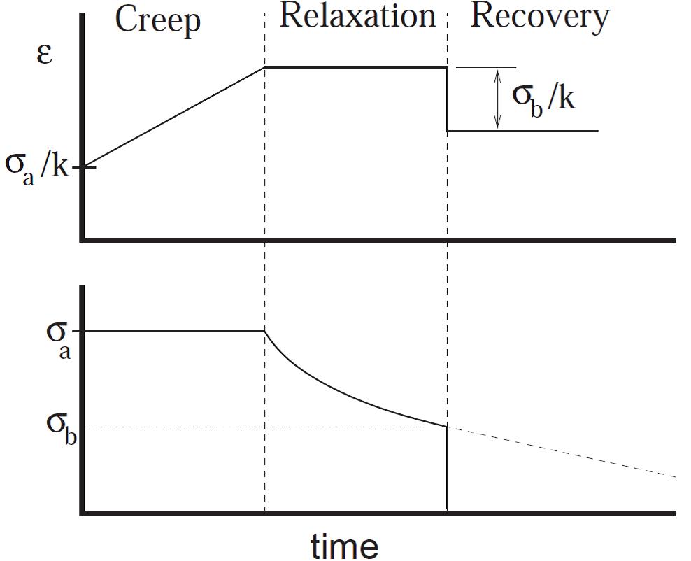

 

 

 

 

 

 

 

 

 

The Maxwell model exhibits an exponential (reversible) stress relaxation and a linear (non reversible) strain creep; it is also referred to as the relaxation element.At the instant of unloading, elastic recovery due to the retreat of the Hookean elastic element is observed and the initial instantaneous strain is entirely recovered.

• Handles Creep badly

• Handles Recovery badly (model only recovers elastic deformation, and does so instantly)

• Accounts fairly well for Relaxation

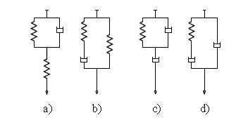
Fig. The mechanical representations of the Zener model, see a), b) and of the anti–Zener model, see c), d), where: a) spring in series with Voigt, b) spring in parallel with Maxwell, c) dashpot in series with Voigt, d) dashpot in parallel with Maxwell.

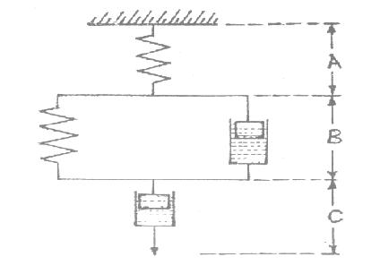
4-Element model (Burgers model):

Burger’smodel-states that the behavior of agricultural materials under stress can be represented by a spring (representing elastic behaviour) in series with a dashpot and a combined spring and a dashpot (representing viscous behaviour) in parallel.

 

Model parameters for different types of fluids:

\[\tau={\tau _o} + K{\dot \gamma ^n}\]

The power law model with or without a yield term has been employed extensively to describe the flow behavior of viscous foods over wide ranges of shear rates where ‘K’ is the consistency coefficient (consistent index, Pa.sⁿ), and ‘n’ is the flow behavior index (dimensionless) is also known as the Herschel-Bulkley model.

t_o=0: (For Newtonian fluid: n=1, Psedoplastic fluid: 0<n<1 and dilatant fluid: n>1) and for plastic fluid: n=0, the flow begins only after a yield stress t_o is reached.

Table 12.1 SI and equivalent rheumatic units

Quantity	SI Unit	Equivalent CGS  unit
viscosity	Pa.s	10 P(poise) or 1000 cP(centipoises)
Kinematic viscosity	m2s-1	104 Stoke or 106 (centistokes)
Shear stress	Pa.s	0.1 dyne.cm-2
strain	unitless	-
Shear rate	s-1	s-1
modulus	Pa	0.1 dyne.cm-2
compliance	Pa-1	10 cm2 dyne-1
frequency	Hz
Angular frequency	2.f
Phase angle	rad

Table 12.2 SI derived units expressed in terms of base units

Symbol	Special name	Other SI Unit	SI base  unit
Pa	Pascal	Nm-2	Kg.m-1s-2
Hz	Hertz	s-1	s-1
rad	Radian		m.m-1

 

References:

Mohsenin, N.N. 1986. Physical Properties of Plant and Animal Materials, 2nd ed.; Gordon and Breach Science Publishers: New York

Sahin S. & Sumnu, S. G. 2006. Physical Properties of Foods. Springer, USA

Abd El-Maksoud, M. A., Gamea, G. R., Abd El-Gawad, A. M. 2009. Rheological constants of the four elements burgers model for potato tubers affected by various fixed loads under different storage conditions. Misr J. Ag. Eng., 26(1): 359- 384