Fluid Mechanics 3(2+1)

LESSON 12. FLUID KINEMATICS

Method of describing Fluid motion

12.2 Lagrangian Description

      1. Lagrangian description of fluid flow tracks the position and velocity of individual particles.

      2. Based upon Newton's laws of motion.

      3. Difficult to use for practical flow analysis.

• Fluids are composed of billions of molecules.
• Interaction between molecules hard to describe/model.

      4. However, useful for specialized applications

• Sprays, particles, bubble dynamics, rarefied gases.
• Coupled Eulerian-Lagrangian methods.

      5. Named after Italian mathematician Joseph Louis Lagrange (1736-1813).

12.3 Eulerian Description

      1. Eulerian description of fluid flow: a flow domain or control volume is defined by which fluid flows in and out.

      2. We define field variables which are functions of space and time.

• Pressure field, P=P(x,y,z,t)
• Velocity field,             \[\vec V=\vec V\left({x,y,z,t}\right)\]

  \[\vec V=u\left({x,y,z,t}\right)\vec i + v\left({x,y,z,t}\right)\vec j+w\left({x,y,z,t}\right)\vec k\]

• Acceleration field,
  

 \[\vec a=\vec a\left({x,y,z,t}\right)\]
\[\vec a=a_x \left({x,y,z,t}\right)\vec i + a_y \left({x,y,z,t}\right)\vec j+a_z \left({x,y,z,t}\right)\vec k\]

• These (and other) field variables define the flow field.

 3. Well suited for formulation of initial boundary-value problems (PDE's).

4. Named after Swiss mathematician Leonhard Euler (1707-1783).

12.4 Coupled Eulerian-Lagrangian Method

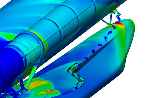
1. Forensic analysis of Columbia accident:  simulation of shuttle debris trajectory using Eulerian CFD for flow field and Lagrangian method for the debris.

12.5 Acceleration Field

1. Consider a fluid particle and Newton's second law,

\[\vec F_{particle}= m_{particle}\vec a_{particle}\]

2.The acceleration of the particle is the time derivative of the particle's velocity.

\[\vec a_{particle}={{d\vec V_{particle}}\over{dt}}\]

3.However, particle velocity at a point is the same as the fluid velocity,

\[\vec V_{particle}= \vec V\left({x_{particle}\left(t\right),y_{particle}\left(t \right),z_{particle}\left(t\right)}\right)\]

4. To take the time derivative of, chain rule must be used.

\[\vec a_{particle}={{\partial\vec V}\over{\partial t}}{{dt}\over{dt}}+{{\partial\vec V}\over{\partial x}}{{dx_{particle}}\over{dt}}+{{\partial\vec V}\over{\partial y}}{{dy_{particle}}\over {dt}}+{{\partial \vec V}\over{\partial z}}{{dz_{particle} }\over {dt}}\]

5. Since

\[{{dx_{particle}}\over {dt}}=u,{{dy_{particle}}\over{dt}}=v,{{dz_{particle}}\over{dt}}=w\]

\[\vec a_{particle}={{\partial\vec V}\over{\partial t}}+ u{{\partial \vec V}\over {\partial x}}+ v{{\partial \vec V}\over{\partial y}}+w{{\partial\vec V}\over{\partial z}}\]

6. In vector form, the acceleration can be written as

\[\vec a\left( {x,y,z,t} \right)={{d\vec V} \over {dt}}={{\partial \vec V} \over {\partial t}} + \left( {\vec V.\vec \nabla } \right)\vec V\]

7. First term is called the local acceleration and is nonzero only for unsteady flows.

8. Second term is called the advective acceleration and accounts for the effect of the fluid particle moving to a new location in the flow, where the velocity is different.

12.6 Material Derivative

1. The total derivative operator d/dt is call the material derivative and is often given special notation, D/DT.

\[{{D\vec V} \over {Dt}}={{d\vec V} \over {dt}}={{\partial \vec V} \over {\partial t}} + \left( {\vec V.\vec \nabla } \right)\vec V\]

2. Advective acceleration is nonlinear:  source of many phenomenon and primary challenge in solving fluid flow problems.

3. Provides ``transformation'' between Lagrangian and Eulerian frames.

4. Other names for the material derivative include:  total, particle, Lagrangian, Eulerian, and substantial derivative.

12.7 Flow visuilization

1. Flow visualization is the visual examination of flow-field features.

2. Important for both physical experiments and numerical (CFD) solutions.

3. Numerous methods

• Streamlines and streamtubes

• Pathlines

• Streaklines

• Timelines

• Refractive techniques

• Surface flow techniques