Food Processing Plant Design & Layout 2(1+1)

Lesson 11. Food processing enterprise

In studying the enterprise's environment one might wish to study in detail the customers, competitors, suppliers, and the legal, political, social and geographic factors which bear upon its operations. To avoid some of the chaos this might involve, it is assumed that all these things can be expressed by the demand curve of the enterprise. The demand curve expresses a part of the relationship of the enterprise with its market by simply giving the amount of product that can be sold as a function of the price charged for it. In this simple model, price is taken to be the major determining factor in the amount the enterprise can sell; and such obvious other factors as quality, advertising, sales effort, reputation, and service are left out of the picture. Thus the relationship between the price and the amount of product that can be sold is given by:

P = a – b D for 0 ≤ D ≤ a/b

= 0 otherwise

Here P is the unit price, D is the amount of product sold, and a and b are positive constants. It is assumed that the amount of product, D, is a continuous variable. The straight-line example, which has been given, might have been a curve; but the point is that one usually expects large volume to be associated with low price, and small volume to be associated with high price (Figure 1).

The analyst who knows the demand curve may then decide what price one will charge, and the curve will tell how much one can sell; or, one may decide what volume to produce and the curve will indicate the highest price at which one will be able to dispose of the production. Ultimately one will make the choice so as to maximize profit, and profit may be defined simply as the difference between total revenue or gross sales (TR) and total cost (TC),

Profit = TR - TC

The total revenue resulting from any price-volume choice may be computed directly from the demand curve.

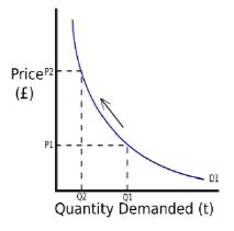
Fig 11.1 A Demand Curve

11.2 Total revenue function

Total revenue of the enterprise is simply the amount of product sold multiplied by the unit price charged. Therefore, 

Total Revenue (TR) = (unit price) (volume) = PD

Where,

P       = unit price, = (a – b D)

D       = amount of product sold, (Volume)

Using the demand function, total revenue can be expressed in terms of D alone,

TR     = (a – b D) D = a D - b D2 for 0 ≤ D ≤ a/b

= 0 otherwise

Now if one were dealing with a peculiar enterprise, which has no costs at all, or has only costs independent of the volume of production, then maximizing profit would be achieved by maximizing total revenue. The volume that will maximize total revenue can be found by the usual methods of calculus (Fig 11.2).

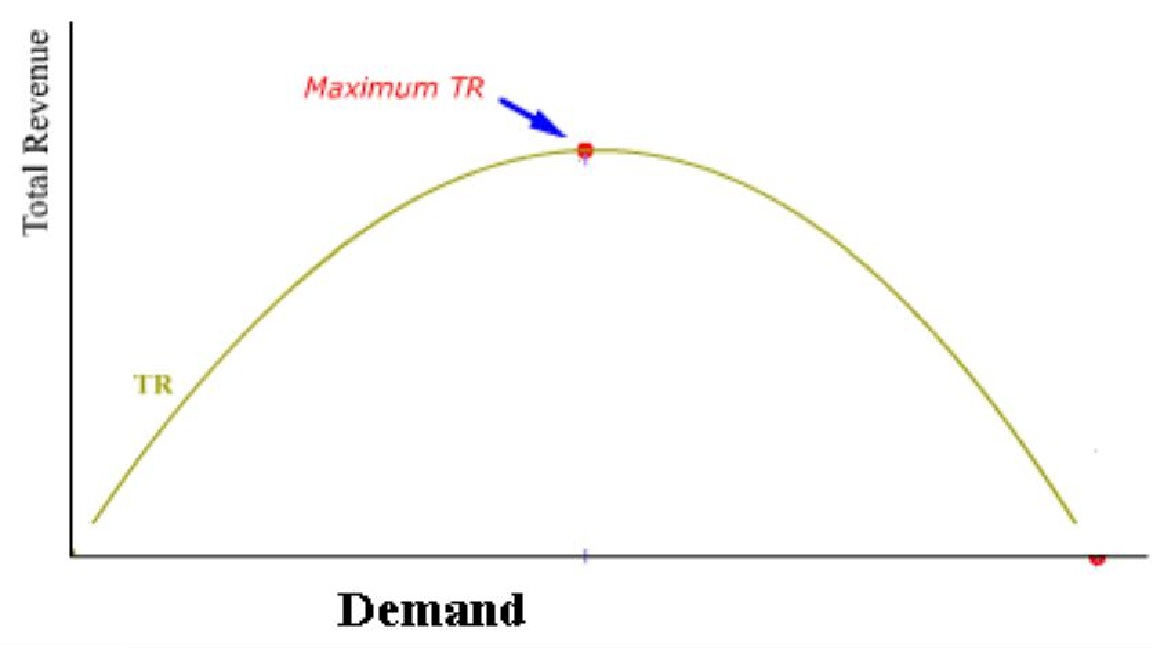
Fig 11.2 A total revenue function

 One may be assured of a maximum by noting that

is negative since b is a positive constant. It may be noted that the derivative of total revenue with respect to volume is given the name "marginal revenue". It expresses the rate at which revenue increases with increase in the volume of sales. Most enterprises, however, would not find that maximum total revenue resulted in maximum profit, thus one must investigate the problem of total cost of production in order to compute the profit in the more usual way.

11.3 Total cost function

Imagine that the analyst is able to examine the productive operations of the enterprise. At this point the analyst may be especially interested in how total cost changes with the volume of production. In estimating total cost it is helpful to divide the components of this sum into two classes called fixed costs and variable costs.

Fixed costs include all costs independent of the volume of production. These are the costs, which must be met irrespective of the level of production.

Variable costs include all costs which vary more or less directly with the volume of production: These costs include such things as direct labour costs and raw material costs that tend to rise as the number of units produced goes up. It may be difficult to discover just exactly how variable costs do 'vary with the level of production. Further, costs which are fixed in the short run may not be fixed in the long run. For example, if production is stopped, the enterprise may meet its fixed expenses for a short period in anticipation of renewed activity, however, this can not go on for long without resulting in liquidation or some other drastic modification of the cost structure. In spite of these difficulties, these cost classifications are sufficiently suggestive to give some important insights. To clarify these, let

TC (D) = total cost at a production level of D units

FC = fixed costs, independent of D

VC (D) = variable costs at a production level of D

TC (D) = FC + VC (D)

This is the general form of the enterprise's total cost function.

Consider a simple case in which the variable cost function turns out to be a simple linear function of the volume of production.

VC (D) = v D

The rate of change of the variable costs with the volume of production is called the "marginal cost," or sometimes the "incremental cost". In this case we have simply

This implies that marginal costs are constant, and that the cost of producing a small additional amount is always the same. If D is taken to be a discrete variable, then the marginal cost is simply the cost of producing one additional unit of product when the production is at some given level.

VC (D + 1) – VC (D) = marginal cost

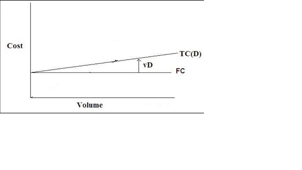
Fig 11.3 A total cost function

Using the simple-linear cost function (Fig 11.3), the total cost function becomes

TC (D) = FC +v D

and profit is given by

Profit = TR (D) – TC (D) = (a D – b D2 ) - (FC +vD)

          = - FC + (a -v) D – bD2 for 0 ≤ D ≤ a/b

   = 0 otherwise

The-analyst who wishes to maximize profit under these conditions will then be interested in the value of D, which maximizes this function. Thus if

a – v ≥ 0 

 

If

a- v ≤ 0 

the profit will be maximized for

D=0

The situation, which confronts the analyst is shown graphically in Fig 11.4, in which it is assumed that

a - v ≥ 0

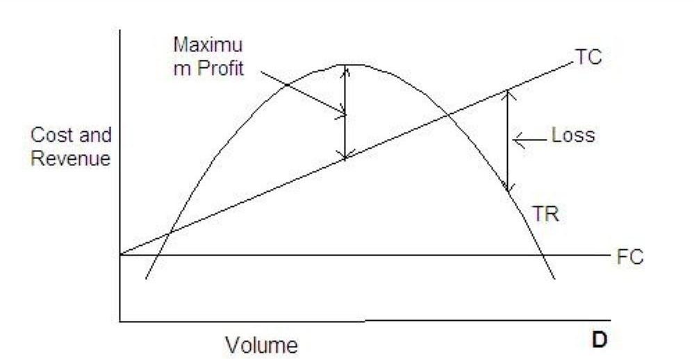
Fig 11.4 A profit - Loss function

An important -principle emerges here if one observes that at this level of production, marginal cost is equal to marginal revenue. For

Thus one might formulate a decision rule which says, “to maximize profit, increase production as long as marginal revenue is greater than marginal cost, but stop when the two are equal”. Alternatively, “to maximize profit, increase production until the revenue from the last unit of product is just equal to the cost of producing it."

11.3 Break-even and shutdown Points

From Fig 11.4 certain other insights may be obtained. There are two points at which total revenue is equal to total cost, and thus profit is zero. These points are called the break- even points. Between the break-even points the enterprise will make a profit, but outside of these it will suffer a loss. The lower or left-hand break-even point is of special interest to the analysts since this is the level of, production that must be reached to get the enterprise out of the red. Many of the decisions of the enterprise about its activities depend heavily on the answer to the question; "Will the venture be able to operate at or above its break-even point?"

Another decision that may confront the analyst is whether or not to cease production entirely when conditions force volume down below the lower break- even point. This decision might be studied using the model, although this is not essential. Suppose the analyst finds that the enterprise is forced to produce at some level lower than the break- even point; one then has the following alternatives:

al = stop production

a2 = continue production at some level D1 below the break-even point

Assuming that no uncertainty or risk is involved in the analysis of this decision, one could compute the profit associated with each alternative:

Profit

a1      - FC

a2      TR (D1) – TC (D1)

The profit for a2 may be computed as follows:

TR (D1) – TC (D1) = TR (D1) – (FC + vD1)

Alternative a2 will be preferred if

TR (D1) - (FC + vD1) > - FC

  TR (D1) > vDl

Thus one has the decision rule, "so long as total revenue exceeds variable costs, do not stop production." This rule must obviously apply in the short run, since the enterprise cannot go on sustaining a loss for very long.

 11.4 Production

The problems and decisions discussed so far are largely the concern of top management, since they are in the realm of major company policy. The analyst at least early in the career, is more likely to be associated with decisions specifically related to the methods of production and operation employed. Thus one may be concerned with alternative production processes, alternative designs for the product, alternative operating procedures, and so on.

Ideally all the decisions should be studied from the overall viewpoint of the enterprise, with the aim of perhaps maximizing total profit as was previously shown. For obvious practical reasons, not every decision can be approached immediately from this viewpoint and thus one uses other, more immediate criteria. Typically much effort is devoted to reducing costs through the improvement of the product, the process, or the operating procedures. Although sometimes it may be true that if costs are reduced by a rupee, profit will increase by a rupee, things are usually not so simple. Suppose, for example, the analyst can show that by refusing to disrupt production in order to push through "rush" orders, costs can be reduced. Clearly profits may not be increased by an equal amount, since the customers may take their business elsewhere. In practice many decisions are approached from the viewpoint of minimizing costs because it may be difficult to measure profit directly, and good judgment indicates that higher profits are likely to result.

11.5 Economics of mass production

Suppose that management is confronted with the following decision. If the production process and equipment are kept substantially the same, what volume of production will minimize the average unit cost of production? This is the question of the economic operating level for a plant. If we assume that under these conditions the plant's costs are given by a linear total cost function, as in Fig 11.5, then the average unit cost is simply given by

 

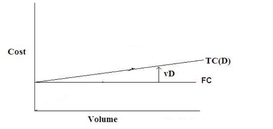
fig 11.5 Atotal cost function

In this situation the more one produces, the lower the average unit cost. This phenomenon is so important that it is given the name "economics of mass production" and forms the entire basis of much of the industrial development. The simple linear cost function leads to the conclusion that production may be increased indefinitely, always with the result of lowering average unit cost. Recalling that the plant and production process is being held substantially constant, this conclusion does not appear realistic. As one tries to obtain more and more production from the plant, the facilities are strained to their limit, expensive overtime operation seems necessary, scrap may increase, maintenance may be neglected and average cost may go up (Fig 11.6).

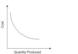
Fig 11.6 an average cost function

This would have been noted, one has assumed a somewhat more realistic total cost function, such as

TC (D) = FC + v1 D + v2 D2 

In this case average cost is given by

and will be minimized when

This yields

The phenomenon of rising average cost which sets in when production goes above this level suggests that we might formulate the general hypothesis: As one tries to get more and more production out of a given plant and process, the unit cost will eventually go up. Thus one has to compromise between the conflicting effects of economies of mass production and the eventual up tuning of the average cost function. The best compromise in the sense of minimizing cost is given by the result obtained above.

At this point, another helpful decision rule may be obtained. At the point where average cost is minimum, it is easy to show that

AC (D) = marginal cost at D = v1 + 2 √ FCv2 

Thus one could say that average cost would come down so long as marginal cost is below it. But when marginal cost exceeds average cost, it will rise. To minimize average cost, find the level of production where it is equal to marginal cost. A little thought will confirm the common sense of this rule.

11.6 A production management decision

The work of the analyst is partly that of transforming management problems into mathematical problems. If the analyst can discover or create a mathematical structure that reasonably reflects the management decision, then he/ she is in a position to use the mathematical structure or model to predict the results of various managerial choices. One way, and perhaps the only way, to become acquainted with the art of model building is to study some examples. Let us take a somewhat more detailed look at production by means of an especially useful model, which may be used to capture some of the complexity of production management decisions. Instead of considering a plant in terms of a production function, we now look more closely at what is inside the plant.

Suppose we have a food processing plant, and our business consists of buying vegetables from farmers, preparing them, and packing them in cans of our own manufacture. The plant consists of three departments: the can department, which produces the containers, the preparation department, which cleans and cooks the vegetables, and the packing department, which fills and labels the cans. At the moment, farmers are offering both peas and tomatoes, either of which could be processed in our plant. Our total cost and revenue structure is so simple that we can say each can of peas yields us a profit of Rs. 5.00 and each can of tomatoes yields a profit of Rs. 8.00. These profits are the same no matter what level of production for either vegetable we decide on if we are planning for the coming week, then our profit for the week will be (in Rupees).

Profit = 6P+8T

where, P is the number of cans of peas we turn out and T is the number of cans of tomatoes. At this point it may appear that since tomatoes are more profitable, we should entirely forsake peas and turn out all the tomatoes possible. However, usually things are not as simple as-that. First of all, we discover that the farmers in the area will have available no more than the equivalent of 20,000 cans of tomatoes and no more than the equivalent of 25,000 cans of peas. Thus our choices of P and T are limited by the availability of vegetables. It must be that

P ≤ 25,000 T ≤ 20,000

Next, we note that the capacity of our departments is also limited. Suppose both vegetables are packed in the same type of can, and the can department has a capacity of 30,000 cans per week. This puts another restriction on our production program.

P + T ≤ 30,000

The preparation department, which operates 40 hours per week, requires 0.001 hours to process enough peas to fill a can and 0.002 hours to process a can of tomatoes. We then have a processing department restriction that says

0.001 P + 0.002 T ≤ 40 

or

P + 2T ≤ 40,000

The packing department has a capacity of 50,000 cans of either type for the week, giving

P + T ≤ 50,000

One might go on adding restrictions and conditions to make the problem more and more realistic, but at this point the decision about a production program is sufficiently complicated to suggest the difficulties that might be encountered.

The problem is still simple enough so that its solution may be graphically illustrated. Any decision as to a production program can be represented by a point on Figure 6, that is, a particular pair of values for P and T. By plotting the inequalities which express the restriction we can see exactly how our choice is limited. Because of the limited production by farmers our choice of P must lie on or below the horizontal line P = 25,000. Similarly, our choice of T must lie to the left of a vertical line T = 20,000. The other two restrictions are similarly plotted, with the result that our decision is limited in fact to P and T combinations lying in or on the edge of the shaded area in Fig 11.7.

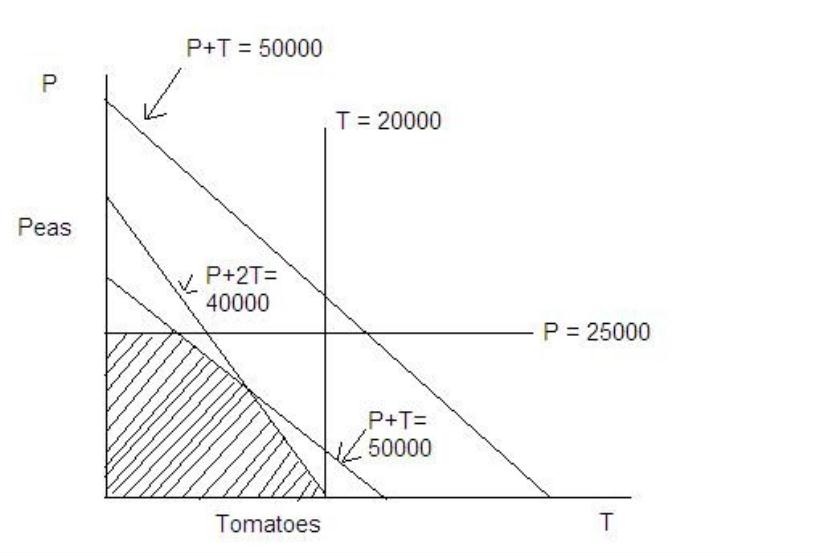
Fig 11.7 Possible production programmes and restrictions

The capacity of the canning department does not need to be considered in this particular decision, since the other restrictions prevent any possibility of reaching this capacity. At the moment we have more capacity than necessary in this department.