Electrical Circuits 3(2+1)

LESSON 5. Loop current and loop equations (Mesh current method)

Figure 5.1 (a) is a planar circuit.  Figure 5.1 (b) is a non-planar circuit and Fig. 5.1 (c) is a planar circuit which looks like a non-planar circuit.  It has already been discussed that a loop is a closed path.  A mesh is defined as a loop which does not contain any other loops within it.  To apply mesh analysis, our first step is to check whether the circuit is planar or not and the second is to select mesh current.  Finally, writing Kirchhoff’s voltage law equations in terms of unknowns and solving them leads to the final solution.

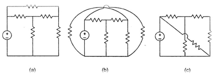
Fig. 5.1

Observation of the Fig.5.2 indicates that there are two loops abefa, and bcdeb in the network.  Let us assume loop currents I₁ and I₂ with directions as indicated in the figure.  Considering the loop abefa alone, we observe that current I₁ is passing through R₁, and (I₁ – I₂) is passing through R₂.  By applying Kirchhoff’s voltage law, we can write

            V_S = I₁R₁ + R₂(I₁ – I₂)

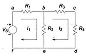
Fig.5.2

Similarly, if we consider the second mesh bcdeb, the current I₂ is passing through R₃ and R₄, and (I₂ -  I₁)  is passing through R₂.  By applying Kirchhoff’s voltage law around the second mesh, we have

            R₂(I₂ – I₁) + R₃ I₂ + R₄ I₂ = 0

By rearranging the above equations, the corresponding mesh current equations are

            I₁(R₁ + R₂) – I₂ R₂ = V_S

            - I₁R₂  + (R₂ + R₃ + R₄)I₂ = 0

By solving the above equations, we can find the currents I₁ and I₂.   If we observe Fig. 5.2, the circuit consists of five branches and four nodes, including the reference node.  The number of mesh currents is equal to the number of mesh equations.

And the number of equations = branches – (nodes -1).  In Fig. 5.2, the required number of mesh currents would be 5 – (4 – 1) = 2.

5.2 Mesh Equations by Inspection Method

The mesh equations for a general planar network can be written by inspection without going through the detailed steps.  Consider a three mesh networks as shown in Fig.5.3.

The loop equations are

            I₁R₁ + R₂(I₁ – I₂) = V_{1 \[...................................................\left( {5.1} \right)\]}

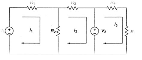
Fig. 5.3

            R₂(I₂ – I₁) = I₂R_{3 = -} V_{2 \[...................................................\left( {5.2} \right)\]}

                        R₄I₃ + R₅I₃ = V_{2 \[...................................................\left( {5.3} \right)\]}

Reordering the above equations, we have

            (R₁ + R₂)I₁ – R₂I_{2 =-} V_{1 \[...................................................\left( {5.4} \right)\]}

            -R₂I₁ + R₂ + R₃) I₂ = - V_{2 \[...................................................\left( {5.5} \right)\]}

                        (R₄ + R₅)I₃ = V_{2 \[...................................................\left( {5.6} \right)\]}

The general mesh equations for three mesh resistive network can be written as

            R₁₁I₁ ± R₁₂I₂ ± R₁₃I₃ = V_{a \[...................................................\left( {5.7} \right)\]}

            ± R₂₁I₁ + R₂₂I₂ ± R₂₃I₃ = V_{b \[...................................................\left( {5.8} \right)\]}

            ± R₃₁I₁ + R₃₂I₂ ± R₃₃I₃ = V_{c \[...................................................\left( {5.9} \right)\]}

By comparing the Eqs. 5.4, 5.5 and 5.6 with Eqs. 5.7, 5.8 and 5.9 respectively, the following observations can be taken into account.

1. The self-resistance in each mesh.
2. The mutual resistances between all pairs of meshes and
3. The algebraic sum of the voltages in each mesh.

The self-resistance of loop 1, R₁₁ = R₁ + R₂, is the sum of the resistances through which I₁ passes. The mutual resistance of loop 1, R₁₂ = - R₂, is the sum of the resistances common to loop currents I₁ and I₂.  If the directions of the currents passing through the common resistance are the same, the mutual resistance will have a positive sign; and if the directions of the currents passing through the common resistance are opposite then the mutual resistance will have a negative sign.

V_a = V₁ is voltage which drives loop one.  Here, the positive sign is used if the direction of the current is the same as the direction of the source.  If the current direction is opposite to the direction of the source, then the negative sign is used.

Similarly, R₂₂ = (R₂ + R₃) and R₃₃ = R₄ + R₅ are the self-resistances of loops two and three, respectively.  The mutual resistances R₁₃ = 0, R₂₁ = - R₂, R₂₃ = 0, R₃₁ = 0, R₃₂ = 0 are the sums of the resistances common to the mesh currents indicated in their subscripts.

V_b = - V₂, V_c = V₂ are the sum of the voltages driving their respective loops.

5.3.  Supermesh Analysis

Suppose any of the branches in the network has a current source, then it is slightly difficult to apply mesh analysis straight forward because first we should assume an unknown voltage across the current source, writing mesh equations as before, and then relate the source current to the assigned mesh currents.  This is generally a difficult approach. One way to overcome this difficulty is by applying the supermesh technique.  Here we have to choose the kind of supermesh.  A supermesh is constituted by two adjacent loops that have a common current source.  As an example, consider the network shown in Fig.5.4.

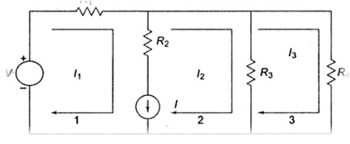
Fig. 5.4

Here, the current source I is in the common boundary for the two meshes 1 and 2.  This current source creates a supermesh, which is nothing but a combination of meshes 1 and 2.

            R₁I₁ + R₃(I₂ – I₃) = V

or         R₁I₁ + R₃I₂ – R₄I₃ = V

Considering mesh 3, we have

            R₃(I₃ – I₂) + R₄I₃ = 0

Finally, the current I from current source is equal to the difference between two mesh currents, i.e..

            I₁ = I₂ = I

We have, thus, formed three mesh equations which we can solve for the three unknown currents in the network.