Electrical Circuits 3(2+1)

LESSON 23. Laplace Transform method of finding step response of DC circuits

\[L\left[ {f\left( t \right)} \right]=F\left( s \right)=\int\limits_{-\infty }^\infty{{e^{-st}}f(t)dt=\int\limits_0^\infty{f(t){e^{-st}}dt}} ...................................................\left( {23.1} \right)\]

is a continuous function for t≥0multiplied by e^-st which is integrated with respect to t between the limits 0 and  ∞.  The resultant function of the variables is called Laplace transform of .  Laplace transform is a function of independent variables corresponding to the complex variable in the exponent of e^-st.  The complex variable S is, in general, of the form S = σ+jω and σ and ω being the real and imaginary parts respectively.  For a function to have a Laplace transform, it must satisfy the condition \[\int\limits_0^\infty{f(t){e^{-st}}dt<\infty.}\] Laplace transform changes the time domain function \[f(t)\] to the frequency domain function F(s).  Similarly, inverse Laplace transformation converts frequency domain function F(s) to the time domain function \[f(t)\]  as follows.

\[{L^{ - 1}}\left[ {F\left( s \right)} \right]=f\left( t \right)={1 \over {2\pi j}}\int\limits_{-j}^{+j} {F(s)\,{e^{st}}\,ds} ...................................................\left( {23.2} \right)\]

Here, the inverse transform involves a complex integration. can be represented as a weighted integral of complex exponentials.  We will denote the transform relationship between \[f(t)\] and F(s) are

\[f(t)\buildrel L \over \longleftrightarrow F(s)\]

In Eq. 23.1, if the lower limit is 0 then the transform is referred to as one sided, or unilateral, Laplace transform.  In the two-sided, or bilateral, Laplace transform, the lower limit is -∞.

In the following discussion, we divide the Laplace transforms into two types:  functional transforms and operational transforms.  A functional transform is the Laplace transform of a specific function, such as sinwt, t, e^-at, and so on.  An operational transform defines a general mathematical property of the Laplace transform, such as binding the transform of the derivative of \[f(t)\] .  Before considering functional and operational transforms, we used to introduce the step and impulse functions.

23.2. Step Function

In switching operations abrupt changes may occur in current and voltages.  On some functions discontinuity may appear at the origin.  We accommodate these discontinuities mathematically by introducing the step and impulse functions. 

Figure 23.1 shows the step function.  It is zero for t<0.  It is denoted by k u (t).

Mathematically it is defined as

k u(t) = 0, t<0

k u(t) = k, t>0 \[...................................................\left( {23.3} \right)\]

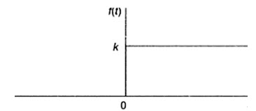
Fig.23.1

If k is 1, the function defined by Eq. (23.3) is the unit step.  The step function is not defined at t=0.  In situations where we need to define the transition between 0 and 0⁺, we assume that it is linear and that

            K u (0) = 0.5 K \[...................................................\left( {23.4} \right)\]

Figure 23.2 shows the linear transition from 0 to 0⁺.

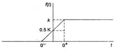
Fig. 23.2

A discontinuity may occur at some time other than t = 0, for example, in sequential switching.  The step function occurring at t = a when a > 0 is shown in Fig.23.3. A step occurs at t = a is expressed as ku(t-a).  thus

            k u(t-a) = 0, t<a

            k u(t-a) = k, t>a \[...................................................\left( {23.5} \right)\]

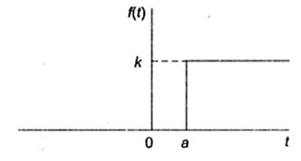
Fig.23.3

If a>0, the step occurs to the right of the origin, and if a<0, the step occurs to the left of the origin.  Step function is 0 when the argument t-a is negative, and it is k when the argument is positive.

A step function equal to k for t<0 is written as ku(a-t).  Thus

            k u(a-t) = k, t<a

            k u(a-t) = 0, t>0 \[...................................................\left( {23.6} \right)\]

The discontinuity is to the left of the origin when a<0.  A step function k u(a-t) for a>0 is shown in Fig.23.4.

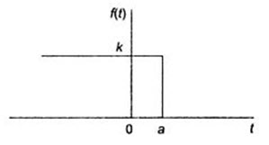
 Fig.23.4

Step function is useful to define a finite-width pulse, by adding two step functions.  For example, the function k[u(t – 1) – u(t – 3)] has the value k or 1<t<3 and the value 0 everywhere else, so it is a finite-width pulse of height k initiated at t = 1 and terminated at t = 3.  Here, u(t – 1) is a function “turning on” the constant value k at t = 1, and the step function –u(t = 3) as “turning off” the constant value k at t = 3.  We use step functions to turn on and turn off linear functions.

23.3 Impulse Function

An impulse is a signal of infinite amplitude and zero duration.  In general, an impulse signal doesn’t exist in nature, but some circuit signals come very close to approximating this definition.  Due to switching operations impulsive voltages and currents occur in circuit analysis.  The impulse function enables us to define the derivative at a discontinuity, and thus to define the Laplace transform of that derivative.

To define derivative of a function at a discontinuity, consider that the function varies linearly across the discontinuity as shown in Fig.23.5.

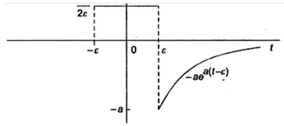
Fig.23.5

In the Fig.23.5 shown as ε→0, an abrupt discontinuity occurs at the origin.  When we differentiate the function, the derivative between -εand +ε is constant at a value of \[{1 \over {2\varepsilon }}\] .  For t>ε, the derivative is –ae^-a(t-ε).  The derivative of the function shown in Fig. 23.5 and shown in Fig.23.6.

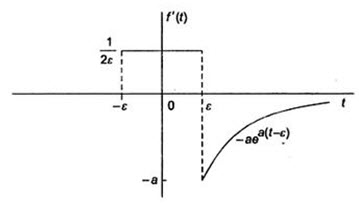
Fig.23.6

As ε approaches zero, the value of \[f'\left( t \right)\] between ±ε approaches infinity.  At the same time, the duration of this large value is approaching zero.  Furthermore, the area under \[f'\left( t \right)\] between ±ε remainsfs constant as ε→0.  In this example, the area is unity.  As ε approaches zero, we say that the function between ±ε approaches a unit impulse function; denoted δ(t).  Thus the derivative of \[f'\left( t \right)\] at the origin approaches a unit impulse function as ε approaches zero, or

\[f\left(0\right)\to\delta\left( t \right)\,\,as\,\,\varepsilon\to 0\]

If the area under the impulse function curve is other than unity, the impulse function is denoted by K δ(t), where K is the area.  K is often referred to as the strength of the impulse function.

Mathematically, the impulse function is defined

\[\int\limits_{-\infty }^\infty{K\,\delta \left(t \right)\,dt = k} ...................................................\left( {23.7} \right)\]

        δ(t) = 0, t ≠ 0 \[...................................................\left( {23.8} \right)\]

Equation (23.7) states that the area under the impulse function is constant.  This area represents the strength of the impulse.  Equation (23.8) states that the impulse is zero everywhere except at t = 0.  An impulse that occurs at t = a is denoted K δ(t – a).  The graphical symbol is shown in Fig.23.7.  The impulse K δ(t-a) is also shown in Fig.23.7.

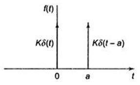
 Fig.23.7

An important property of the impulse function is the shifting property, which is expressed as

\[\int\limits_{-\infty }^\infty{f\left( t \right)\,\delta \left({t - a} \right)\,dt=f\left( a \right)} ...................................................\left( {23.9} \right)\]

Equation 23.19 shows that the impulse function shifts out everything except the value of \[f\left( t \right)\] at t = a.  The value of δ(t-a) is zero everywhere except at t=a, and hence the integral can be written

\[I=\int\limits_{-\infty}^\infty{f\left(t\right)\,\delta\left({t-a}\right)\,dt=\int\limits_{a-\in}^{a+\in}{f\left(t\right)\,\delta\left({t-a}\right)dt}} ...................................................\left( {23.10} \right)\]

But because \[f\left( t \right)\] is continuous at a, it takes on the value \[f\left( a \right)\] as t → a, so

\[I=\int\limits_{a-\in }^{a+ \in }{f\left(a\right)\,\delta \left({t - a} \right)\,dt = f\left( a \right)\int\limits_{a - \in }^{a + \in }{\,\delta \left({t - a} \right)dt=f\left( a \right)} } ...................................................\left( {23.11} \right)\]

We use the shifting property of the impulse function to find its Laplace transform.

\[L\left[ {\delta \left( t \right)} \right]=\int\limits_{0-}^\infty{\delta \left( t \right){e^{-st}}\,\,dt=\int\limits_{0-}^\infty{\delta \left( t \right)\,\,dt = 1} } ...................................................\left( {23.12} \right)\]

which is important Laplace transform pair that we make good use of the circuit analysis. 

We can also define the derivatives of the impulse function and the Laplace transform of these derivatives.           

The function illustrated in Fig.23.8 (a) generates an impulse function as ε→0.  Figure 23.8 (b) shows the derivative of the impulse generating function, which is defined as the derivative of the impulse [δ’(t)] as ε→0.  The derivative of the impulse function sometimes is referred to as a moment function, or unit doublet.

To find the Laplace transform of δ’(t), we simply apply the defining integral to the function shown in Fig.23.6 (b) and, after integrating, let ε→ 0.  Then,

\[L\left\{ {\delta '\left( t \right)} \right\}=\lim \left[ {\int\limits_{-\varepsilon }^0 {{1 \over 2}{e^{-st\,}}\,dt}+\int\limits_{{0^ +}}^\varepsilon{\left({{{-1} \over {{\varepsilon ^2}}}} \right){e^{ - st}}\,\,dt} } \right]\]

\[=\,\,\lim \,\,{{{e^{s\varepsilon }} + {e^{ - s\varepsilon }} - 2} \over {s{\varepsilon ^2}}}\]

\[=\,\,\lim \,\,{{s{e^{s\varepsilon }} - {e^{ - s\varepsilon }}} \over {2\varepsilon s}}\]

\[= \,\,\lim \,\,{{{s^2}{e^{s\varepsilon }} + {s^2}{e^{ - s\varepsilon }}} \over {2s}}\]

\[=s...................................................\left( {23.13} \right)\]

Fig.23.8(a)                                          Fig.23.8(b)

For the nth derivative of the impulse, we find that its Laplace transform simply is sⁿ; that

is , \[L\left\{ {\delta '\left( t \right)} \right\} = {s^n}...................................................\left( {23.14} \right)\]

An impulse function can be thought of as a derivative of a step function, that is

\[\delta \left( t \right)={{du\left( t \right)} \over {dt}}...................................................\left( {23.15} \right)\]

Figure 23.9 (a) approaches a unit step function as ε→ 0.  The function shown in Fig. 23.9 (b), the derivative of the function in 23.9 (b), approaches a unit impulse as ε→ 0.

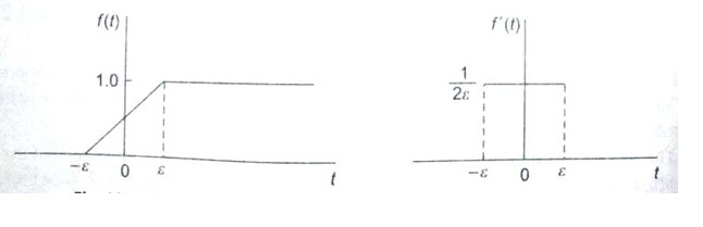
 Fig.23.9 (a)                                         Fig.23.9 (b)

The impulse function is an extremely useful concept in circuit analysis where discontinuities occur at the origin.