Site pages
Current course
Participants
General
Module 1. Average and effective value of sinusoida...
Module 2. Independent and dependent sources, loop ...
Module 3. Node voltage and node equations (Nodal v...
Module 4. Network theorems Thevenin’ s, Norton’ s,...
Module 5. Reciprocity and Maximum power transfer
Module 6. Star- Delta conversion solution of DC ci...
Module 7. Sinusoidal steady state response of circ...
Module 8. Instantaneous and average power, power f...
Module 9. Concept and analysis of balanced polypha...
Module 10. Laplace transform method of finding ste...
Module 11. Series and parallel resonance
Module 12. Classification of filters
Module 13. Constant-k, m-derived, terminating half...
LESSON 25. Laplace Transform of Periodic Functions and inverse transforms
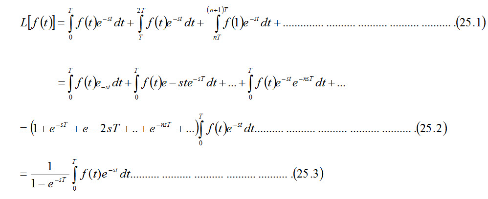
25.1. Laplace Transform of Periodic Functions
Periodic functions appear in many practical problems. Let function \[f(t)\] be a periodic function which satisfies the condition \[f(t)\] = \[f(t + T)\] for all t>0 where T is period of the function.
25.2 Inverse Transforms
So far, we have discussed Laplace transform of functions \[f(t)\] . If the function is a rational function of s, which can be expressed in the form of a ratio of two polynomial in s such that no non-integral powers of s appear in the polynomials. In fact, for liner, lumped parameter circuits whose component values are constant, the s-domain expressions for the unknown voltages and currents are always rational functions of s. If we can inverse transform rational functions of s, we can solve for the time domain expressions for the voltages and currents.
In general, we need to find the inverse transform of a function that has the form.
\[F\left( s \right) = {{N\left( s \right)} \over {D\left( s \right)}}={{{a_n}{s^n} + {a_{n - 1}}{s^{n - 1}} + ..... + {a_1}s + {a_0}} \over {{b_m}{s^m} + {b_{m - 1}}{s^{m - 1}} + .... + {b_1}s + {b_0}}}...................................................\left( {25.4} \right)\]
The coefficients a and b are real constants, and the exponents m and n are positive integers. The ratio \[{{N\left( 2 \right)} \over {D\left( 2 \right)}}\] is called a paper rational function if m>n, and an improper rational function if m ≤ n. Only a proper rational function can be expanded as a sum of partial fractions.
Partial Fraction Expansion: Proper Rational Functions
A proper rational function is expanded into a sum of partial fractions by writing a term or a series of terms for each root of D(s). Thus D(s) must be in factored form before we can make a particle fraction expansion. The roots of D(s) are either (1) real and distinct (2) complex and distinct (3) real and repeated or (H) complex and repeated.
When the roots are real and distinct
In this case \[F\left( s \right)={{N\left( s \right)} \over {D\left( s \right)}}...................................................\left( {25.5} \right)\]
Where D(s) = (s-a) (s-b) (s-c) \[...................................................\left( {25.6} \right)\]
Expanding F(s) into partial fractions, we get
\[F(s)={A \over {s - a}} + {B \over {s - b}} + {C \over {s - c}}...................................................\left( {25.7} \right)\]
To obtain the constant A, multiplying Eq. (25.7) with (s-a) and putting s = a, we get
\[F(s)\,(s - a)\,{\,_{s = a}}=A\]
Similarly, we can get the other constants,
\[B=(s - b)\,\,F{(s)_{s = b}}\]
\[C=(s - c)\,\,F{(s)_{s = c}}\]
When roots are real and repeated
In this case \[F\left( {s={{N\left( s \right)} \over {D\left( s \right)}}} \right)\]
where \[D\left( s \right)={\left( {s - a} \right)^n}\,\,{D_1}\left( s \right)\]
The partial fraction expansion of F(s) is
\[F\left( s \right)={{{A_0}} \over {{{\left( {s - a} \right)}^n}}} + {{{A_1}} \over {{{\left( {s - a} \right)}^{n - 1}}}} + ... + {{{A_{n - 1}}} \over {s - a}} + {{{N_1}\left( s \right)} \over {{D_1}\left( s \right)}}...................................................\left( {25.8} \right)\]
Where \[{{{N_1}\left( s \right)} \over {{D_1}\left( s \right)}}\] represents the remainder terms of expansion.
To obtain the constant A0’ A1’ … An-1’ let us multiply both sides of Eq.(25.8) by (s-a)n.
Thus
(s – a)n F(s) = F1(s) = A0 + A1 (s – a) + A2 (s – a)2 + …
+An-1 (s – a)n-1 + R(s) (s – a)n \[.....................\left( {25.9} \right)\]
Where R(s) indicates the remainder terms
Putting s = a, we get
A0 = (s – a)n F(s)/s=a
Differentiating Eq. (13.117) with respect to s, and putting s = a, we get
\[{A_1}={d \over {ds}}{F_1}\left( s \right){|_{s = a}}\]
Similarly, \[{A_2}={1 \over {2!}}{{{d^2}} \over {d{s^2}}}{F_1}\left( s \right){|_{s = a}}\]
In general, \[{A_n}={\left. {{1 \over {n!}}{{{d^n}{F_1}\left( s \right)} \over {d{s^n}}}} \right|_{s = a}}...................................................\left( {25.10} \right)\]
When roots are distinct complex roots of D(s)
Consider a function
\[[F\left(s\right)={{N\left(s\right)}\over{D\left(s\right)\left({s-\alpha+j\beta}\right)\left({s-\alpha-j\beta}\right)}}...................................................\left( {25.11} \right)\]
The partial fraction expansion of F(s) is
\[F\left(s\right)={A\over{s-\alpha-j\beta}}+{B\over{s-\alpha+j\beta}}+{{{N_1}\left(s \right)} \over {{D_1}\left( s \right)}}...................................................\left( {25.12} \right)\]
where \[{{{N_1}\left( s \right)} \over {{D_1}\left( s \right)}}\] is the remainder term.
Multiplying Eq. (25.12) by (s-a-jβ) and putting
S = a + jβ.
we get \[A={{N\left({\alpha+j\beta }\right)}\over{{D_1}\left({\alpha+j\beta}\right)\left({+2j\beta}\right)}}...................................................\left( {25.13} \right)\]
Similarly \[B={{N\left({\alpha+j\beta } \right)} \over {\left({-2j\beta}\right){D_1}\left({\alpha-\beta } \right)}}...................................................\left( {25.14} \right)\]
In general, B = A* where A* is complex conjugate of A.
If we denote the inverse transform of the complex conjugate terms as ƒ (t)
\[f\left( t \right)={L^{ - 1}}\left[ {{A \over {s - \alpha- j\beta }} + {B \over {s - \alpha+j\beta }}} \right]...................................................\left( {25.15} \right)\]
\[={L^{ - 1}}\left[ {{A \over {s - \alpha-j\beta }} + {B \over {s - \alpha+j\beta }}} \right]\]
where A and A* are conjugate terms.
If we denote A = C+jD, then
B = C – jD = A*
f(t) = eat (Aejβt + A* e-jβt)
When roots are repeated and complex of D(s)
The complex roots always appear in conjugate pairs and that the coefficients associated with a conjugate pair are also conjugate, so that only half the Ks need to be evolved.
Consider the function \[F\left( s \right)={{768} \over {{{\left( {{s^2} + 6s + 2s} \right)}^2}}}...................................................\left( {25.17} \right)\]
By factoring the denominator polynomial, we have
\[F\left( s \right)={{768} \over {{{\left( {s + 3 - j4} \right)}^2}{{\left( {s + 3 + j4} \right)}^2}}}\]
\[={{{K_1}} \over {{{\left( {s + 3 - j4} \right)}^2}}} + {{{K_2}} \over {s + 3 - j4}}\]
\[+ {{K_1^*} \over {{{\left( {s + 3 + j4} \right)}^2}}} + {{K_2^*} \over {s + 3 + j4}}...................................................\left( {25.18} \right)\]
Now we need to evaluate only K1 and K2 because K*1 and K*2 are conjugate values. The value of K1’ is
\[K1={\left.{{{768}\over{{{\left({s+3+j4}\right)}^2}}}}\right|_{s=-3+j4}}={{768}\over{{{\left({j8}\right)}^2}}}=-12...................................................\left( {25.19} \right)\]
The value of K2 is
\[K2={d \over {ds}}{\left[ {{{768} \over {{{\left( {s + 3 + j4} \right)}^2}}}} \right]_{s=-3+j4}}\]
\[=-{\left. {{{2\left({768}\right)}\over{{{\left({s+3+j4}\right)}^3}}}}\right|_{s=-3 + j4}}=-{{2\left( {768} \right)}\over {{{\left( {j8} \right)}^3}}}\]
![]() .................................................\left( {25.20} \right)\]
.................................................\left( {25.20} \right)\]
Partial Fraction Expansion: Improper Rational Function
An improper rational function can always be expanded into a polynomial plus a proper rational function. The polynomial is then inverse –transformed into impulse functions and derivatives of impulse functions.
\[F\left( s \right)={{{S^4} + 13_s^3 + 66_s^2 + {{200}_s} + 300} \over {{s^2} + 9s + 20}}...................................................\left( {25.21} \right)\]
Dividing the denominator into the numerator until the remainder is proper rational function gives
\[F\left( s \right)={s^2} + 4s + 10 + {{30s + 100} \over {{s^2} + 9s + 20}}...................................................\left( {25.22} \right)\]
Now we expand the proper rational function into a sum of partial fractions
\[{{30s + 100} \over {{s^2} + 9s + 20}}={{30s + 100} \over {\left( {s + 4} \right)\,\,\left( { + 5} \right)}} = {{ - 20} \over {s + 4}} + {{50} \over {s + 5}}...................................................\left( {25.23} \right)\]
Substituting Eq. (25.23) into Eq. (25.22) yields
\[F\left( s \right)={s^2} + 4s + 10 - {{20} \over {s + 4}} + {{50} \over {s + 5}}...................................................\left( {25.24} \right)\]
By taking inverse transform, we get
\[f\left( t \right)={{{d^2}\delta \left( t \right)} \over {d{t^2}}} + 4{{d\delta \left( t \right)} \over {dt}} + 10\,\,\delta \left( t \right) - \left( {20{e^{ - 4t}} - 50{e^{ - 5t}}} \right)u\left( t \right)...................................................\left( {25.25} \right)\]
25.3. Initial and Final Value Theorems
The initial and final value theorems are useful because they enable us to determine from \[F\left( s \right)\] the behavior of \[f\left( t \right)\] at 0 and ∞. Hence we can check the initial and final value of to sec if they conform with known circuit behavior, before actually finding the inverse transform of \[F\left( s \right)\].
The initial –value theorem states that
\[\lim \,f\left( t \right)=\lim SF(s)...................................................\left( {25.26} \right)\]
and the final-value theorem states that
\[\lim \,f\left( t \right)=\lim SF(s)...................................................\left( {25.27} \right)\]
The initial-value theorem is based on the assumption that contains no impulse functions.
To prove, initial value theorem, we start with the operational transform of the fits derivative.
\[L\left[ {{{df} \over {dt}}} \right]=SF\left( s \right) - f\left( 0 \right)\]
\[=\int\limits_0^\infty{{{df} \over {dt}}{e^{ - st}}dt} ...................................................\left( {25.28} \right)\]
Now we take the limit as → ∞
\[{\lim }\limits_{s \to \infty} \left[ {SF\left( {s - f\left( 0 \right)} \right)} \right]={\lim }\limits_{s \to \infty } \int\limits_0^\infty{{{df} \over {dt}}} {e^{ - st}}\,\,dt...................................................\left( {25.29} \right)\]
The right hand side of the above equation becomes zero as s®¥
\[{\lim }\limits_{s \to \infty} \left[ {SF\left( s \right) - f\left( 0 \right)} \right]= 0\]
\[{\lim }\limits_{s \to \infty} SF\left( s \right) = f\left( 0 \right)={\lim }\limits_{s \to \infty} f\left( t \right)...................................................\left( {25.30} \right)\]
The proof of the final value theorem also starts with Eq. (25.31). Here we take the limit as s→0.
\[{\lim }\limits_{s \to \infty} \left[ {SF\left(s\right)-f\left( 0 \right)} \right]={\lim }\limits_{s \to 0} s\left( {\int\limits_0^\infty{{{df} \over {dt}}{e^{ - st}}\,dt} } \right)...................................................\left( {25.31} \right)\]
\[{\lim }\limits_{s \to 0} \left[ {SF\left( s \right) - f\left( 0 \right)} \right] = \left[ {f\left( t \right)} \right]_0^\infty ...................................................\left( {25.32} \right)\]
\[{\lim }\limits_{s \to 0} \left[ {SF\left( s \right) - f\left( 0 \right)} \right]={\lim }\limits_{t \to \infty} \,f\left( t \right) - f\left( 0 \right)\]
Since \[f\left( 0 \right)\] is not a function of s, it gets cancelled from both sides.
\[{\lim }\limits_{t \to \infty } f\left( t \right)={\lim }\limits_{s \to 0} \,FS\left( 0 \right)...................................................\left( {25.33} \right)\]
The final-value theorem is useful only if \[f\left( \infty\right)\] exists.
Application of initial and final value theorems
Consider the transform pair given by
\[{{100\left( {s + 3} \right)} \over {\left( {s + 6} \right)\left( {{s^2} + 6s + 25} \right)}} \leftrightarrow \left[ {212{e^{ - 6t}} + 20{e^{ - 3t}}\cos \left( {4t - {{53.13}^0}} \right)} \right]\,u\left( t \right)........................................\left( {25.34} \right)\]
The initial value theorem gives
\[{\lim}\limits_{s\to\infty}\left[{SF\left(s\right)={\lim}\limits_{s\to\infty}}\right]\frac{{100{s^2}\left({1+\frac{3}{s}}\right)}}{{{s^3}\left[{1+\frac{6}{s}}\right]\left[{1+\frac{6}{s}+\frac{{25}}{{{s^2}}}}\right]}}=0.............\left({25.35}\right)\]
\[{\lim}\limits_{t\to 0}f\left(t\right)=\left[{-12+20\cos\left({-{{53.13}^0}} \right)} \right]\left( 1 \right)=-12 + 12 = 0...................................................\left( {25.36} \right)\]
The final value theorem gives
\[{\lim }\limits_{s \to 0} \,SF\left( s \right)={\lim }\limits_{s \to 0} {{100s\left( {s + 3} \right)} \over {\left( {s + 6} \right)\left( {{s^2} + 6s + 25} \right)}} = 0...................................................\left( {25.37} \right)\]
\[{\lim }\limits_{t \to \infty } \,f\left( t \right)={\lim }\limits_{t \to \infty} \left[ { - 12{e^{ - 6t}} + 20{e^{ - 3t}}\cos \left( {4t - {{53.13}^0}} \right)} \right]u\left( t \right) = 0...................................................\left( {25.38} \right)\]
Last modified: Wednesday, 13 November 2013, 7:18 AM