Electrical Circuits 3(2+1)

LESSON 30. Constant-k filters

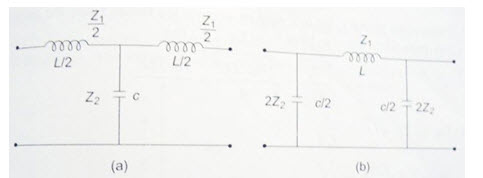
Fig. 30.1

Fig.30.1 (a) and (b), where Z₁ = jω_L and Z₂ = 1/jω_C.  Hence Z₁Z₂= \[{L \over C}={k^2}\] which is independent of frequency.

\[{Z_1}{Z_2}={k^2}={L \over C}\,\,\,or\,\,k=\sqrt {{L \over C}} ...................................................\left( {30.2} \right)\]

Since the product Z₁ and Z₂ is constant, the filter is a constant-k  type.  From Eq. 29.8 (a) the cut-off frequencies are Z₁/4Z₂ = 0.

i.e.          \[{{ - {\omega ^2}LC} \over 4}=0\]

i.e.         \[f=0\,\,and\,\,{{{Z_1}} \over {4{Z_2}}}=-1\]

               \[{{ - {\omega ^2}LC} \over 4}=-1\]

or           \[{f_c}={1 \over {\pi \sqrt {LC} }}...................................................\left( {30.3} \right)\]

The pass band can be determined graphically.  The reactances of Z₁ and 4Z₂ will vary with frequency as drawn in Fig.30.2.  The cut-off frequency at the intersection of the curves Z₁ and 4Z₂ is indicated as ƒ_c.  On the X-axis as Z₁ = -4Z₂ at cut-off frequency, the pass band lies between the frequencies at which Z₁ = 0, and Z₁=-4Z₂.

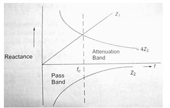
Fig.30.2

All the frequencies above ƒ_c lie in a stop or attenuation band.  Thus, the network is called a low-pass filter.  We also have from Eq.28.7 (previous chapter) that

\[\sinh {\gamma\over 2}=\sqrt {{{{Z_1}} \over {4{Z_2}}}}=\sqrt {{{ - {\omega ^2}LC} \over 4}}={{J\omega \sqrt {LC} } \over 2}\]

From Eq. 30.3 \[\sqrt {LC}={1 \over {{f_c}\pi }}\]

\[\sinh {\gamma\over 2}={{j2\pi f} \over {2\pi {f_c}}}=j{f \over {{f_c}}}\]

We also know that in the pass band

                       \[-1<{{{Z_1}} \over {4{Z_2}}}< 0\]

                       \[-1<{{ - {\omega ^2}LC} \over 4}< 0\]

                       \[-1<-\left( {{f \over {{f_c}}}} \right)< 0\]

or                    \[{f \over {{f_c}}} < 1\]

and                 \[\beta=2{\sin ^{ - 1}}\left( {{f \over {{f_c}}}} \right);\,\,\alpha=0\]

In the attenuation band,

                       \[{{{Z_1}} \over {4{Z_2}}}<-1,\,\,i.e.{f \over {{f_c}}} < 1\]

                       \[\alpha=2{\cosh ^{ - 1}}\left[ {{{{Z_1}} \over {4{Z_2}}}} \right]=2{\cosh ^{ - 1}}\left[ {{f \over {{f_c}}}} \right];\,\beta=\pi\]

The plots of \[\alpha\] and β for pass and stop bands are shown in Fig.30.3.

Thus, from Fig.30.3, a = 0, b = 2 sinh^-1 \[\left( {{f \over {{f_c}}}} \right)for\,\,f < {f_c}\]

                       \[\alpha=2{\cosh ^{ - 1}}\left( {{f \over {{f_c}}}} \right);\,\beta=\pi \,\,for\,\,f > fc\,\,f < {f_c}\]

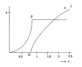
Fig.30.3

The characteristic impedance can be calculated as follows.

\[{Z_{0T}}=\sqrt {{Z_1}{Z_2}\left( {1 + {{{Z_1}} \over {4{Z_2}}}} \right)}\]

       \[=\sqrt {{L \over C}\left( {1 + {{{\omega ^2}LC} \over 4}} \right)}\]

\[{Z_{0T}}=k{\sqrt {1 - \left( {{f \over {{f_c}}}} \right)} ^2}...................................................\left( {30.4} \right)\]

 From Eq.30.4, Z_0T is real when ƒ < ƒ_c i.e. in the pass band at ƒ = ƒ_c, Z_0T = 0; and for ƒ > ƒ_c, Z_0T is imaginary in the attenuation band, rising to infinite reactance at infinite frequency.  The variation of Z_0T with frequency is shown in Fig.30.4.

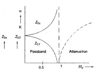
Fig.30.4

Similarly, the characteristic impedance of a \[\pi\]-network is given by

                       

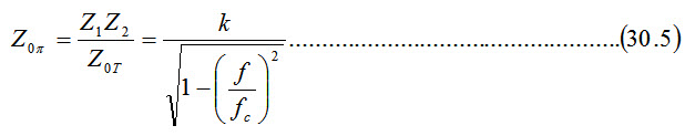
The variation of Z_0\[\pi\] with frequency is shown in fig. 30.4 for ƒ< ƒ_c, Z_0\[\pi\] is real; at ƒ = ƒ_c, Z_0\[\pi\] is infinite, and for ƒ > ƒ_c, Z_0T is imaginary.  A low pass filter can be designed from the specifications of cut-off frequency and load resistance.

All cut-off frequency, Z₁= -4Z₂

                       \[j{\omega _c}L={{ - 4} \over {j{\omega _c}C}}\]

                       \[{\pi ^2}f_c^2LC=1\]

Also we know that \[k=\sqrt {L/C}\]  is called the design impedance or the load resistance

\[{k_2}={L \over C}\]

\[{\pi ^2}f_c^2{k^2}{C^2}=1\]

\[C={1 \over {\pi \,{f_c}k}}\,gives\,\,the\,\,value\,\,of\,\,the\,\,shunt\,capaci\tan ce\]

\[and\,L={k^2}C={k \over {\pi {f_c}}}\,gives\,the\,value\,of\,the\,series\,induc\tan ce.\]

30.2. Constant K-High Pass Filter

Constant K-high pass filter can be obtained by changing the positions of series and shunt arms of the networks shown in Fig.30.1.  The prototype high pass filters are shown in Fig.30.5, where Z₁ =-j/ω_C and Z₂ = jωL.

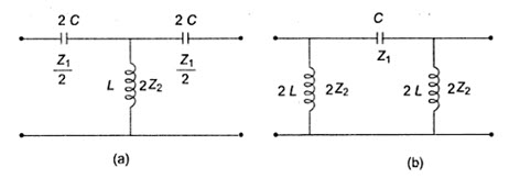
Fig.30.5

Again, it can be observed that the product of Z₁ and Z₂ is independent of frequency, and the filter design obtained will be of the constant k type.  Thus, Z₁Z₂ are given by

\[{Z_1}{Z_2}={{ - j} \over {\omega C}}j\omega L={L \over C}={k^2}\]

The cut-off frequencies are given by Z₁= 0 and Z₁ =-4Z₂.

\[{Z_1}\,=\,0\,indicates\,{j \over {\omega C}}=0,\,\,or\,\,\omega\to \alpha\]

From Z₁ =-4Z₂

             \[{{ - j} \over {\omega C}}=-4j\omega L\]

             \[{\omega ^2}LC={1 \over 4}\]

or         \[{f_c}={1 \over {4\pi \sqrt {LC} }}...................................................\left( {30.6} \right)\]

The reactance of Z₁ and Z₂ are sketched as functions of frequency as shown in Fig.30.6.

As seen from Fig.30.6, the filter transmits all frequencies between ƒ = ƒ_c and ƒ = \[\propto\]  .  The point ƒ_c from the graph is a point at which Z₁ = -4Z₂.

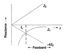
Fig.30.6

                \[\sinh {\gamma\over 2}=\sqrt {{{{Z_1}} \over {4{Z_2}}}}=\sqrt {{{ - 1} \over {4{\omega ^2}LC}}}\]

                 \[From\,Eq.17.25,{f_c}={1 \over {4\pi \sqrt {LC} }}\]

           \[\sqrt {LC}={1 \over {4\pi {f_c}}}\]

           \[\sinh {\gamma\over 2}=\sqrt {{{ - {{\left( {4\pi } \right)}^2}{{\left( {{f_c}} \right)}^2}} \over {4{\omega ^2}}}}=j{{{f_c}} \over f}\]

In the pass band, \[- 1 < {{{Z_1}} \over {4{Z_2}}} < 0,\alpha=0\,\,or\,the\,region\,which\,{{{f_c}} \over f} < 1\,is\,a\,pass\,band\]

\[\beta=2{\sin ^{ - 1}}\left( {{{{f_c}} \over f}} \right)\]

In the attenuation band \[{{{Z_1}} \over {4{Z_2}}}<-1,i.e.{{{f_c}} \over f} > 1\]

                       \[\alpha=2{\cosh ^{ - 1}}\left( {{{{Z_1}} \over {4{Z_2}}}} \right)\]

                       \[=2{\cos ^{ - 1}}\left( {{{{f_c}} \over f}} \right);\,\,\beta=-\pi\]

The plots of a and b for pass and stop bands of a high pass filter network are shown in Fig.30.7

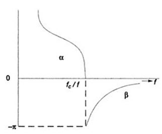Fig.30.7

A high pass filter may be designed similar to the low pass filter by choosing a resistive load r equal to the constant k, such that \[R=k=\sqrt {L/C}\]

        \[{f_c}={1 \over {4\pi \sqrt {L/C} }}\]

         \[{f_c}={k \over {4\pi L}}={1 \over {4\pi Ck}}\]

Since      \[\sqrt C={L \over k},\]

                 \[L={k \over {4\pi {f_c}}}and\,C={1 \over {4\pi {f_c}k}}\]

The characteristic impedance can be calculated using the relation

                \[{Z_{0T}}=\sqrt {{Z_1}{Z_2}\left( {1 + {{{Z_1}} \over {4{Z_2}}}} \right)}=\sqrt {{L \over C}\left( {1 - {1 \over {4{\omega ^2}LC}}} \right)}\]

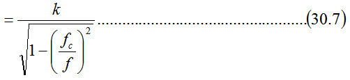
         \[{Z_{0T}}=k\sqrt {1 - {{\left( {{{{f_c}} \over f}} \right)}^2}}\]

Similarly, the characteristic impedance of a p-network is given by

                 \[{Z_{0\pi }}={{{Z_1}{Z_2}} \over {{Z_{0T}}}}={{{k_2}} \over {{Z_{0T}}}}\]

                       

The plot of characteristic impedance with respect to frequency is shown in Fig.30.8

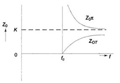
Fig.30.8